🌊 Random Forest: Deep Dive & Best Practices

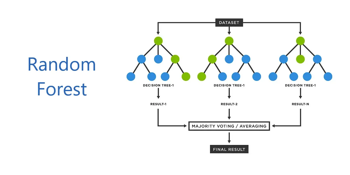
Table of Contents

1. Introduction
2. Core Concepts
   1. Ensemble Learning
   2. Decision Trees Foundation
3. Algorithm Workflow
   1. Training Process
   2. Prediction Process
4. Terminology Tables
   1. Table 1: Process Stage Terminology
   2. Table 2: Component Hierarchy
   3. Table 3: Data Flow Terminology
5. Hyperparameters
   1. Critical Hyperparameters
      1. n_estimators
      2. max_features
      3. max_depth
      4. min_samples_split
      5. min_samples_leaf
      6. bootstrap
      7. oob_score
   2. Supporting Hyperparameters
      1. random_state
      2. n_jobs
      3. criterion
6. Feature Importance
   1. Methods
      1. 1. Mean Decrease in Impurity (MDI)
      2. 2. Permutation Feature Importance
      3. 3. SHAP Values
   2. Python Implementation
7. Out-of-Bag (OOB) Error
   1. Concept
   2. Advantages
   3. Limitations
   4. Python Implementation
8. Hyperparameter Tuning
   1. Tuning Strategies
      1. 1. Grid Search
      2. 2. Randomized Search
      3. 3. Bayesian Optimization
   2. Best Practices for Tuning
9. Complete Implementation Examples
   1. Classification Example
   2. Regression Example
10. Advantages
11. Limitations and When to Avoid
    1. Limitations
    2. When NOT to Use Random Forest
12. Best Practices
    1. Data Preparation
    2. Model Training
    3. Model Evaluation
    4. Optimization
    5. Production Deployment
13. Common Pitfalls and Solutions
    1. Pitfall 1: Too Few Trees
    2. Pitfall 2: Deep Overfitting
    3. Pitfall 3: Ignoring Class Imbalance
    4. Pitfall 4: Not Using OOB Score
    5. Pitfall 5: Inappropriate Feature Preprocessing
    6. Pitfall 6: Treating as Online Learner
    7. Pitfall 7: Misinterpreting Feature Importance
14. Advanced Techniques
    1. 1. Handling Imbalanced Data
    2. 2. Probability Calibration
    3. 3. Partial Dependence Plots
    4. 4. Stacking with Random Forest
    5. 5. Multi-output Random Forest
15. Comparison with Other Algorithms
    1. Random Forest vs Gradient Boosting
    2. Random Forest vs Decision Tree
    3. Random Forest vs Neural Networks
16. Mathematical Foundation
    1. Gini Impurity
    2. Entropy (Information Gain)
    3. Variance Reduction (Regression)
    4. Bootstrap Sample Probability
    5. Feature Importance Formula
17. Real-World Applications
    1. 1. Healthcare
    2. 2. Finance
    3. 3. E-commerce
    4. 4. Agriculture
    5. 5. Environmental Science
    6. 6. Manufacturing
18. Debugging and Troubleshooting
    1. Problem: Poor Performance
    2. Problem: Slow Training
    3. Problem: High Memory Usage
    4. Problem: Inconsistent Results
19. Performance Optimization Checklist
    1. Training Phase
    2. Prediction Phase
    3. Memory Management
    4. Code Quality
20. Summary
21. References

---

Introduction

Random Forest is a powerful ensemble learning algorithm that combines multiple decision trees to produce accurate and robust predictions. Developed by Leo Breiman and Adele Cutler in 2001, it has become one of the most widely-used machine learning algorithms due to its simplicity, versatility, and strong performance across diverse applications.

Random Forest works by constructing numerous decision trees during training and outputting the mode of classes for classification tasks or the mean prediction for regression tasks. This ensemble approach significantly reduces overfitting and variance compared to individual decision trees.

---

Core Concepts

Ensemble Learning

Ensemble learning combines predictions from multiple models to achieve better performance than any single model. Random Forest employs two key ensemble techniques:

Bagging (Bootstrap Aggregating): Each tree is trained on a random sample (bootstrap sample) drawn with replacement from the original training data. Approximately 67% of the data is included in each bootstrap sample, leaving about 33% as out-of-bag samples for validation.

Feature Randomness: At each node split, only a random subset of features is considered for finding the best split, rather than evaluating all features. This decorrelates the trees and reduces variance.

Decision Trees Foundation

Before understanding Random Forests, it is essential to grasp decision trees. A decision tree is a supervised learning algorithm that recursively splits data based on feature values to minimize impurity at each node.

Splitting Criteria:

• Classification: Gini impurity or Information Gain (entropy)
• Regression: Variance reduction

Decision trees are prone to overfitting when grown to maximum depth, capturing noise and specific patterns from training data. Random Forests address this by averaging multiple deep trees.

---

Algorithm Workflow

Training Process

Step 1: Bootstrap Sampling

For each tree \(t\) in the forest (where \(t = 1, 2, ..., N\)):

• Draw \(n\) samples with replacement from the training set of size \(n\)
• This creates a bootstrap sample where approximately 63.2% are unique samples
• The remaining ~36.8% form the out-of-bag (OOB) set for that tree

Step 2: Random Feature Selection

At each node during tree construction:

• Randomly select \(m\) features from total \(p\) features (\(m < p\))
• Default values:
  • Classification: \(m = \sqrt{p}\)
  • Regression: \(m = p/3\)
• Find the best split among these \(m\) features only

Step 3: Tree Growing

• Grow each tree to maximum depth without pruning
• Each tree makes its own independent prediction
• No cross-tree communication during training

Step 4: Aggregation

For predictions:

• Classification: Majority voting across all trees
• Regression: Mean of predictions from all trees

Prediction Process

Given a new input \(x\):

Classification:

\[\hat{y} = \text{mode}\{h_1(x), h_2(x), ..., h_N(x)\}\]

where \(h_i(x)\) is the prediction from tree \(i\)

Regression:

\[\hat{y} = \frac{1}{N}\sum_{i=1}^{N} h_i(x)\]

---

Terminology Tables

Table 1: Process Stage Terminology

General Term	Random Forest Specific	Ensemble Context	Statistical Context	Alternative Terms
Training	Forest Construction	Ensemble Building	Model Fitting	Learning Phase
Sampling	Bootstrap Sampling	Bagging	Resampling with Replacement	Data Aggregation
Splitting	Node Splitting	Feature Selection	Recursive Partitioning	Tree Growing
Aggregation	Voting/Averaging	Ensemble Combination	Prediction Pooling	Consensus Building
Validation	OOB Evaluation	Internal Validation	Holdout Testing	Cross-validation
Prediction	Inference	Ensemble Prediction	Forward Pass	Scoring

Table 2: Component Hierarchy

Level	Component	Description	Scope
1 (Highest)	Random Forest	Complete ensemble model	Entire algorithm
2	Individual Trees	Decision tree estimators	Single classifier/regressor
3	Tree Structure	Nodes and branches	Tree architecture
4	Node	Split point	Single decision
5	Split	Feature threshold	Binary partition
6 (Lowest)	Leaf	Terminal prediction	Final output node

Table 3: Data Flow Terminology

Stage	Input	Process	Output	Alternative Names
Initialization	Original Dataset	Bootstrap Sampling	Training Subsets	Data Preparation
Tree Construction	Bootstrap Sample	Recursive Splitting	Decision Tree	Model Building
Feature Selection	All Features	Random Sampling	Feature Subset	Attribute Sampling
Node Processing	Parent Node	Split Evaluation	Child Nodes	Branching
Aggregation	Tree Predictions	Voting/Averaging	Final Prediction	Ensemble Output

---

Hyperparameters

Critical Hyperparameters

n_estimators

• Description: Number of trees in the forest
• Default: 100 (scikit-learn)
• Impact: More trees improve accuracy but increase computational cost
• Best Practice: Start with 100-500; increase until performance plateaus
• Range: 50-1000+ depending on dataset size

max_features

• Description: Number of features to consider for best split at each node
• Default:
  • Classification: 'sqrt' (\(\sqrt{n_{features}}\))
  • Regression: 'log2' or 1.0 (all features)
• Options: 'sqrt', 'log2', None, integer, or float
• Impact: Controls tree correlation and randomness
• Best Practice: Use defaults; tune only if overfitting occurs

max_depth

• Description: Maximum depth of each tree
• Default: None (nodes expand until pure or min_samples_split reached)
• Impact: Deeper trees capture complex patterns but may overfit
• Best Practice: Start with None; limit if overfitting or high memory usage

min_samples_split

• Description: Minimum samples required to split an internal node
• Default: 2
• Impact: Higher values prevent overfitting to small groups
• Best Practice: 2-20; increase for noisy data

min_samples_leaf

• Description: Minimum samples required at a leaf node
• Default: 1
• Impact: Smooths predictions; prevents overly specific leaves
• Best Practice: 1-10; higher for smoother decision boundaries

bootstrap

• Description: Whether to use bootstrap sampling
• Default: True
• Impact: Enables bagging and OOB evaluation
• Best Practice: Keep True for standard random forest

oob_score

• Description: Whether to calculate out-of-bag score
• Default: False
• Impact: Provides internal validation metric
• Best Practice: Set True for quick model assessment

Supporting Hyperparameters

random_state

• Description: Controls randomness for reproducibility
• Default: None
• Best Practice: Set to fixed integer (e.g., 42) for reproducible results

n_jobs

• Description: Number of parallel jobs
• Default: None (single processor)
• Options: -1 (all processors), 1, or specific number
• Best Practice: Use -1 for large datasets to leverage multicore processing

criterion

• Description: Split quality measure
• Default:
  • Classification: 'gini'
  • Regression: 'squared_error'
• Options:
  • Classification: 'gini', 'entropy', 'log_loss'
  • Regression: 'squared_error', 'absolute_error', 'friedman_mse', 'poisson'
• Best Practice: Defaults work well; experiment if domain-specific

---

Feature Importance

Random Forest provides built-in feature importance measures to identify which features contribute most to predictions.

Methods

1. Mean Decrease in Impurity (MDI)

Also called Gini importance. Calculates total reduction in node impurity weighted by probability of reaching that node across all trees.

Computation: For feature \(j\):

\[\text{Importance}(j) = \frac{1}{N}\sum_{t=1}^{N}\sum_{k \in \text{tree}_t} p_k \Delta i(k, j)\]

where:

• \(N\) = number of trees
• \(p_k\) = proportion of samples reaching node \(k\)
• \(\Delta i(k, j)\) = decrease in impurity at node \(k\) using feature \(j\)

Advantages:

• Fast computation (calculated during training)
• Built into scikit-learn via feature_importances_ attribute

Limitations:

• Biased toward high-cardinality features (many unique values)
• Can overestimate importance of continuous features
• Based on training data only

2. Permutation Feature Importance

Measures decrease in model performance when a feature’s values are randomly shuffled.

Algorithm:

1. Calculate baseline performance on validation set
2. For each feature:
   • Randomly shuffle feature values
   • Calculate new performance
   • Importance = baseline performance - shuffled performance
3. Repeat multiple times and average

Advantages:

• Model-agnostic (works with any model)
• Not biased toward high-cardinality features
• Uses holdout/validation data

Limitations:

• Computationally expensive
• Slower than MDI

3. SHAP Values

SHAP (SHapley Additive exPlanations) provides both global and local feature importance based on game theory.

Advantages:

• Consistent and theoretically sound
• Provides local explanations for individual predictions
• Handles feature interactions

Limitations:

• Computationally intensive
• Requires external library (shap)

Python Implementation

import numpy as np
import pandas as pd
from sklearn.ensemble import RandomForestClassifier
from sklearn.model_selection import train_test_split
from sklearn.inspection import permutation_importance
import matplotlib.pyplot as plt

# Load data
from sklearn.datasets import load_iris
X, y = load_iris(return_X_y=True)
feature_names = load_iris().feature_names

# Split data
X_train, X_test, y_train, y_test = train_test_split(
    X, y, test_size=0.3, random_state=42
)

# Train model
rf = RandomForestClassifier(n_estimators=100, random_state=42)
rf.fit(X_train, y_train)

# Method 1: MDI (Gini Importance)
importances_mdi = rf.feature_importances_
std = np.std([tree.feature_importances_ for tree in rf.estimators_], axis=0)

# Create DataFrame for visualization
importance_df = pd.DataFrame({
    'Feature': feature_names,
    'Importance': importances_mdi,
    'Std': std
}).sort_values('Importance', ascending=False)

print("Mean Decrease in Impurity:")
print(importance_df)

# Plot MDI
plt.figure(figsize=(10, 6))
plt.barh(importance_df['Feature'], importance_df['Importance'])
plt.xlabel('Feature Importance')
plt.title('Feature Importance (Mean Decrease in Impurity)')
plt.tight_layout()
plt.show()

# Method 2: Permutation Importance
perm_importance = permutation_importance(
    rf, X_test, y_test, n_repeats=10, random_state=42, n_jobs=-1
)

perm_df = pd.DataFrame({
    'Feature': feature_names,
    'Importance': perm_importance.importances_mean,
    'Std': perm_importance.importances_std
}).sort_values('Importance', ascending=False)

print("\nPermutation Importance:")
print(perm_df)

# Plot Permutation Importance
plt.figure(figsize=(10, 6))
plt.barh(perm_df['Feature'], perm_df['Importance'])
plt.xlabel('Permutation Importance')
plt.title('Feature Importance (Permutation Method)')
plt.tight_layout()
plt.show()

---

Out-of-Bag (OOB) Error

Out-of-Bag error provides an internal validation mechanism unique to bagging-based algorithms like Random Forest.

Concept

When training with bootstrap sampling, approximately 36.8% of samples are left out for each tree. These out-of-bag (OOB) samples act as a validation set for that specific tree.

OOB Score Calculation:

1. For each sample \(i\) in training set:
   • Identify trees where sample \(i\) was out-of-bag
   • Aggregate predictions from these trees only
   • Compare with true label
2. Calculate accuracy across all samples:

\[\text{OOB Score} = \frac{\text{Correct OOB predictions}}{\text{Total samples}}\]

Advantages

• Free validation: No need for separate validation set
• Efficient: Computed during training without extra cost
• Unbiased estimate: Approximates cross-validation error
• Maximizes data usage: All data used for training

Limitations

• Only available when bootstrap=True
• May overestimate error in certain conditions:
  • Small sample sizes
  • Balanced class distributions
  • High number of features relative to samples

Python Implementation

from sklearn.ensemble import RandomForestClassifier
from sklearn.datasets import make_classification
import matplotlib.pyplot as plt

# Generate synthetic data
X, y = make_classification(
    n_samples=1000, 
    n_features=20, 
    n_informative=15,
    n_redundant=5,
    random_state=42
)

# Track OOB error as trees are added
oob_errors = []
n_trees_range = range(10, 201, 10)

for n_trees in n_trees_range:
    rf = RandomForestClassifier(
        n_estimators=n_trees,
        oob_score=True,
        random_state=42,
        n_jobs=-1
    )
    rf.fit(X, y)
    
    oob_error = 1 - rf.oob_score_
    oob_errors.append(oob_error)
    print(f"Trees: {n_trees}, OOB Error: {oob_error:.4f}")

# Plot OOB error convergence
plt.figure(figsize=(10, 6))
plt.plot(n_trees_range, oob_errors, marker='o')
plt.xlabel('Number of Trees')
plt.ylabel('OOB Error Rate')
plt.title('Out-of-Bag Error vs Number of Trees')
plt.grid(True)
plt.tight_layout()
plt.show()

Comparison with Cross-Validation:

from sklearn.model_selection import cross_val_score

# OOB Score
rf_oob = RandomForestClassifier(
    n_estimators=100, 
    oob_score=True, 
    random_state=42
)
rf_oob.fit(X, y)
print(f"OOB Score: {rf_oob.oob_score_:.4f}")

# Cross-Validation Score
rf_cv = RandomForestClassifier(n_estimators=100, random_state=42)
cv_scores = cross_val_score(rf_cv, X, y, cv=5)
print(f"CV Score: {cv_scores.mean():.4f} ± {cv_scores.std():.4f}")

---

Hyperparameter Tuning

Tuning Strategies

1. Grid Search

Exhaustively searches through a manually specified subset of hyperparameter space.

Advantages:

• Comprehensive search within specified range
• Guaranteed to find best combination in grid

Disadvantages:

• Computationally expensive
• Inefficient for large hyperparameter spaces

from sklearn.model_selection import GridSearchCV
from sklearn.ensemble import RandomForestClassifier

# Define parameter grid
param_grid = {
    'n_estimators': [100, 200, 300],
    'max_depth': [10, 20, 30, None],
    'min_samples_split': [2, 5, 10],
    'min_samples_leaf': [1, 2, 4],
    'max_features': ['sqrt', 'log2']
}

# Initialize Random Forest
rf = RandomForestClassifier(random_state=42)

# Grid search with cross-validation
grid_search = GridSearchCV(
    estimator=rf,
    param_grid=param_grid,
    cv=5,
    n_jobs=-1,
    verbose=2,
    scoring='accuracy'
)

# Fit grid search
grid_search.fit(X_train, y_train)

# Best parameters
print("Best Parameters:", grid_search.best_params_)
print("Best CV Score:", grid_search.best_score_)

# Best model
best_rf = grid_search.best_estimator_

2. Randomized Search

Samples random combinations from hyperparameter distributions.

Advantages:

• More efficient than grid search
• Can explore wider range
• Good for initial exploration

Disadvantages:

• May miss optimal combination
• Requires more iterations for convergence

from sklearn.model_selection import RandomizedSearchCV
from scipy.stats import randint, uniform

# Define parameter distributions
param_distributions = {
    'n_estimators': randint(100, 500),
    'max_depth': [10, 20, 30, None],
    'min_samples_split': randint(2, 20),
    'min_samples_leaf': randint(1, 10),
    'max_features': ['sqrt', 'log2', None],
    'bootstrap': [True, False]
}

# Initialize Random Forest
rf = RandomForestClassifier(random_state=42)

# Randomized search
random_search = RandomizedSearchCV(
    estimator=rf,
    param_distributions=param_distributions,
    n_iter=100,  # number of random combinations
    cv=5,
    n_jobs=-1,
    verbose=2,
    random_state=42,
    scoring='accuracy'
)

# Fit randomized search
random_search.fit(X_train, y_train)

# Results
print("Best Parameters:", random_search.best_params_)
print("Best CV Score:", random_search.best_score_)

3. Bayesian Optimization

Uses probabilistic model to guide search toward promising regions.

Advantages:

• Most efficient for expensive evaluations
• Learns from previous iterations
• Better than random search with fewer iterations

Disadvantages:

• Requires additional library
• More complex to implement

from skopt import BayesSearchCV
from skopt.space import Real, Categorical, Integer

# Define search space
search_spaces = {
    'n_estimators': Integer(100, 500),
    'max_depth': Integer(10, 50),
    'min_samples_split': Integer(2, 20),
    'min_samples_leaf': Integer(1, 10),
    'max_features': Categorical(['sqrt', 'log2']),
}

# Initialize Bayesian optimization
bayes_search = BayesSearchCV(
    estimator=RandomForestClassifier(random_state=42),
    search_spaces=search_spaces,
    n_iter=50,
    cv=5,
    n_jobs=-1,
    verbose=2,
    random_state=42
)

# Fit Bayesian search
bayes_search.fit(X_train, y_train)

print("Best Parameters:", bayes_search.best_params_)
print("Best CV Score:", bayes_search.best_score_)

Best Practices for Tuning

1. Start with defaults: Random Forest works well with default parameters
2. Prioritize tuning order:
   • First: n_estimators, max_features
   • Second: max_depth, min_samples_split, min_samples_leaf
   • Last: Other parameters
3. Use appropriate CV folds: 5-fold for most cases; 10-fold for small datasets
4. Balance accuracy vs computational cost: More trees and deeper trees = slower
5. Monitor overfitting: Check training vs validation scores
6. Use OOB score for quick validation: Faster than CV during exploration

---

Complete Implementation Examples

Classification Example

import numpy as np
import pandas as pd
from sklearn.datasets import load_breast_cancer
from sklearn.model_selection import train_test_split, cross_val_score
from sklearn.ensemble import RandomForestClassifier
from sklearn.metrics import (
    classification_report, 
    confusion_matrix, 
    roc_auc_score,
    roc_curve
)
import matplotlib.pyplot as plt
import seaborn as sns

# Load data
data = load_breast_cancer()
X, y = data.data, data.target
feature_names = data.feature_names

# Split data
X_train, X_test, y_train, y_test = train_test_split(
    X, y, test_size=0.2, random_state=42, stratify=y
)

print(f"Training samples: {X_train.shape[0]}")
print(f"Testing samples: {X_test.shape[0]}")
print(f"Number of features: {X_train.shape[1]}")

# Initialize Random Forest Classifier
rf_clf = RandomForestClassifier(
    n_estimators=200,
    max_depth=20,
    min_samples_split=5,
    min_samples_leaf=2,
    max_features='sqrt',
    bootstrap=True,
    oob_score=True,
    random_state=42,
    n_jobs=-1,
    verbose=1
)

# Train model
print("\nTraining Random Forest Classifier...")
rf_clf.fit(X_train, y_train)

# OOB Score
print(f"\nOOB Score: {rf_clf.oob_score_:.4f}")

# Cross-validation
cv_scores = cross_val_score(
    rf_clf, X_train, y_train, cv=5, scoring='accuracy'
)
print(f"CV Accuracy: {cv_scores.mean():.4f} ± {cv_scores.std():.4f}")

# Predictions
y_pred = rf_clf.predict(X_test)
y_pred_proba = rf_clf.predict_proba(X_test)[:, 1]

# Evaluation
print("\nClassification Report:")
print(classification_report(y_test, y_pred, target_names=data.target_names))

# Confusion Matrix
cm = confusion_matrix(y_test, y_pred)
plt.figure(figsize=(8, 6))
sns.heatmap(cm, annot=True, fmt='d', cmap='Blues', 
            xticklabels=data.target_names,
            yticklabels=data.target_names)
plt.title('Confusion Matrix')
plt.ylabel('True Label')
plt.xlabel('Predicted Label')
plt.tight_layout()
plt.show()

# ROC Curve
fpr, tpr, thresholds = roc_curve(y_test, y_pred_proba)
roc_auc = roc_auc_score(y_test, y_pred_proba)

plt.figure(figsize=(8, 6))
plt.plot(fpr, tpr, color='darkorange', lw=2, 
         label=f'ROC curve (AUC = {roc_auc:.2f})')
plt.plot([0, 1], [0, 1], color='navy', lw=2, linestyle='--')
plt.xlim([0.0, 1.0])
plt.ylim([0.0, 1.05])
plt.xlabel('False Positive Rate')
plt.ylabel('True Positive Rate')
plt.title('Receiver Operating Characteristic (ROC) Curve')
plt.legend(loc="lower right")
plt.grid(alpha=0.3)
plt.tight_layout()
plt.show()

# Feature Importance
importances = rf_clf.feature_importances_
indices = np.argsort(importances)[::-1][:10]  # Top 10 features

plt.figure(figsize=(12, 6))
plt.title('Top 10 Feature Importances')
plt.bar(range(10), importances[indices])
plt.xticks(range(10), [feature_names[i] for i in indices], rotation=45, ha='right')
plt.ylabel('Importance')
plt.tight_layout()
plt.show()

Regression Example

import numpy as np
import pandas as pd
from sklearn.datasets import load_diabetes
from sklearn.model_selection import train_test_split, cross_val_score
from sklearn.ensemble import RandomForestRegressor
from sklearn.metrics import (
    mean_squared_error, 
    mean_absolute_error, 
    r2_score
)
import matplotlib.pyplot as plt

# Load data
data = load_diabetes()
X, y = data.data, data.target
feature_names = data.feature_names

# Split data
X_train, X_test, y_train, y_test = train_test_split(
    X, y, test_size=0.2, random_state=42
)

print(f"Training samples: {X_train.shape[0]}")
print(f"Testing samples: {X_test.shape[0]}")

# Initialize Random Forest Regressor
rf_reg = RandomForestRegressor(
    n_estimators=200,
    max_depth=15,
    min_samples_split=5,
    min_samples_leaf=2,
    max_features='sqrt',
    bootstrap=True,
    oob_score=True,
    random_state=42,
    n_jobs=-1,
    verbose=1
)

# Train model
print("\nTraining Random Forest Regressor...")
rf_reg.fit(X_train, y_train)

# OOB Score
print(f"\nOOB Score (R²): {rf_reg.oob_score_:.4f}")

# Cross-validation
cv_scores = cross_val_score(
    rf_reg, X_train, y_train, cv=5, scoring='r2'
)
print(f"CV R² Score: {cv_scores.mean():.4f} ± {cv_scores.std():.4f}")

# Predictions
y_pred = rf_reg.predict(X_test)

# Evaluation
mse = mean_squared_error(y_test, y_pred)
rmse = np.sqrt(mse)
mae = mean_absolute_error(y_test, y_pred)
r2 = r2_score(y_test, y_pred)

print(f"\nTest Set Performance:")
print(f"RMSE: {rmse:.2f}")
print(f"MAE: {mae:.2f}")
print(f"R² Score: {r2:.4f}")

# Prediction vs Actual Plot
plt.figure(figsize=(10, 6))
plt.scatter(y_test, y_pred, alpha=0.6, edgecolors='k')
plt.plot([y_test.min(), y_test.max()], 
         [y_test.min(), y_test.max()], 
         'r--', lw=2)
plt.xlabel('Actual Values')
plt.ylabel('Predicted Values')
plt.title('Random Forest Regression: Predicted vs Actual')
plt.grid(alpha=0.3)
plt.tight_layout()
plt.show()

# Residuals Plot
residuals = y_test - y_pred
plt.figure(figsize=(10, 6))
plt.scatter(y_pred, residuals, alpha=0.6, edgecolors='k')
plt.axhline(y=0, color='r', linestyle='--', lw=2)
plt.xlabel('Predicted Values')
plt.ylabel('Residuals')
plt.title('Residual Plot')
plt.grid(alpha=0.3)
plt.tight_layout()
plt.show()

# Feature Importance
importances = rf_reg.feature_importances_
indices = np.argsort(importances)[::-1]

plt.figure(figsize=(10, 6))
plt.title('Feature Importances')
plt.bar(range(len(importances)), importances[indices])
plt.xticks(range(len(importances)), 
           [feature_names[i] for i in indices], 
           rotation=45, ha='right')
plt.ylabel('Importance')
plt.tight_layout()
plt.show()

---

Advantages

1. High Accuracy: Ensemble approach produces superior predictions compared to individual trees
2. Robust to Overfitting: Averaging multiple trees reduces variance and prevents overfitting
3. Handles Missing Data: Can maintain performance with missing values through surrogate splits
4. No Feature Scaling Required: Tree-based nature makes it invariant to feature scaling
5. Feature Importance: Provides interpretable feature importance scores
6. Versatility: Works for both classification and regression tasks
7. Non-parametric: Makes no assumptions about data distribution
8. Parallel Processing: Trees can be trained independently, enabling multicore computation
9. Built-in Validation: OOB error provides unbiased performance estimate
10. Resistant to Outliers: Ensemble voting reduces impact of extreme values

---

Limitations and When to Avoid

Limitations

1. Computational Cost: Training many deep trees is memory and time-intensive
2. Prediction Speed: Slower inference compared to simpler models; evaluating all trees takes time
3. Model Interpretability: Black-box nature makes it harder to explain than single decision trees
4. Memory Requirements: Storing entire forest requires significant memory
5. Extrapolation Issues: Cannot predict values outside training range in regression tasks
6. Linear Relationships: May underperform on purely linear data compared to linear models
7. High-Cardinality Bias: Feature importance can be biased toward features with many unique values
8. Not Incremental: Cannot update model with new data; requires complete retraining

When NOT to Use Random Forest

1. Real-time Prediction Requirements

• Low-latency applications where millisecond response times are critical
• Consider: Linear models, shallow decision trees, or optimized neural networks

2. Limited Computational Resources

• Memory-constrained devices or embedded systems
• Consider: Logistic regression, Naive Bayes, or single decision tree

3. Linear Relationships

• Data with clear linear patterns
• Consider: Linear regression, Ridge, Lasso

4. High Interpretability Required

• Regulatory compliance requiring explainable decisions
• Medical diagnosis where decision paths must be transparent
• Consider: Single decision tree, linear models, or rule-based systems

5. Online Learning Needed

• Streaming data requiring incremental updates
• Consider: Online gradient descent, incremental decision trees

6. Time Series Forecasting

• Temporal dependencies requiring sequential modeling
• Cannot extrapolate trends beyond training data
• Consider: ARIMA, Prophet, LSTM, or specialized time series models

7. Very Small Datasets

• Fewer than 100-200 samples
• Risk of overfitting despite ensemble approach
• Consider: Regularized linear models, k-NN

8. Extremely Large Datasets

• Datasets with millions of samples and features
• Training time becomes prohibitive
• Consider: Gradient boosting (XGBoost, LightGBM), or neural networks with mini-batch training

---

Best Practices

Data Preparation

1. Handle Missing Values

from sklearn.impute import SimpleImputer

# For numerical features
imputer_num = SimpleImputer(strategy='median')
X_num = imputer_num.fit_transform(X_numerical)

# For categorical features
imputer_cat = SimpleImputer(strategy='most_frequent')
X_cat = imputer_cat.fit_transform(X_categorical)

2. No Feature Scaling Needed

• Random Forest is invariant to feature scaling
• Skip normalization/standardization for efficiency

3. Encode Categorical Variables

from sklearn.preprocessing import LabelEncoder, OneHotEncoder

# Binary categorical: LabelEncoder
le = LabelEncoder()
X['binary_feature'] = le.fit_transform(X['binary_feature'])

# Multi-class categorical: OneHotEncoder
ohe = OneHotEncoder(sparse_output=False, handle_unknown='ignore')
X_encoded = ohe.fit_transform(X[['categorical_feature']])

4. Balance Classes (for Classification)

from imblearn.over_sampling import SMOTE
from imblearn.under_sampling import RandomUnderSampler

# For imbalanced datasets
smote = SMOTE(random_state=42)
X_balanced, y_balanced = smote.fit_resample(X_train, y_train)

# Or use class_weight parameter
rf = RandomForestClassifier(class_weight='balanced')

Model Training

1. Start with Defaults

rf = RandomForestClassifier(
    n_estimators=100,
    random_state=42,
    n_jobs=-1
)

2. Monitor Training

# Track training progress
rf = RandomForestClassifier(verbose=1)
rf.fit(X_train, y_train)

3. Use Stratified Splitting (Classification)

from sklearn.model_selection import train_test_split

X_train, X_test, y_train, y_test = train_test_split(
    X, y, test_size=0.2, stratify=y, random_state=42
)

4. Enable OOB Scoring

rf = RandomForestClassifier(
    oob_score=True,
    bootstrap=True
)
rf.fit(X_train, y_train)
print(f"OOB Score: {rf.oob_score_}")

Model Evaluation

1. Multiple Metrics

from sklearn.metrics import accuracy_score, precision_score, recall_score, f1_score

y_pred = rf.predict(X_test)

print(f"Accuracy: {accuracy_score(y_test, y_pred):.4f}")
print(f"Precision: {precision_score(y_test, y_pred, average='weighted'):.4f}")
print(f"Recall: {recall_score(y_test, y_pred, average='weighted'):.4f}")
print(f"F1 Score: {f1_score(y_test, y_pred, average='weighted'):.4f}")

2. Cross-Validation

from sklearn.model_selection import cross_validate

# Multiple scoring metrics
scoring = ['accuracy', 'precision_weighted', 'recall_weighted', 'f1_weighted']

scores = cross_validate(
    rf, X, y, cv=5, scoring=scoring, n_jobs=-1
)

for metric in scoring:
    print(f"{metric}: {scores[f'test_{metric}'].mean():.4f} ± {scores[f'test_{metric}'].std():.4f}")

3. Learning Curves

from sklearn.model_selection import learning_curve

train_sizes, train_scores, val_scores = learning_curve(
    rf, X, y, cv=5, n_jobs=-1,
    train_sizes=np.linspace(0.1, 1.0, 10),
    scoring='accuracy'
)

# Plot learning curves
plt.figure(figsize=(10, 6))
plt.plot(train_sizes, train_scores.mean(axis=1), label='Training score')
plt.plot(train_sizes, val_scores.mean(axis=1), label='Validation score')
plt.xlabel('Training Set Size')
plt.ylabel('Score')
plt.legend()
plt.title('Learning Curves')
plt.grid(alpha=0.3)
plt.tight_layout()
plt.show()

Optimization

1. Incremental Tuning

# Step 1: Tune n_estimators
for n in [50, 100, 200, 300]:
    rf = RandomForestClassifier(n_estimators=n, random_state=42)
    scores = cross_val_score(rf, X_train, y_train, cv=5)
    print(f"n_estimators={n}: {scores.mean():.4f}")

# Step 2: Tune max_features
for mf in ['sqrt', 'log2', None]:
    rf = RandomForestClassifier(n_estimators=200, max_features=mf, random_state=42)
    scores = cross_val_score(rf, X_train, y_train, cv=5)
    print(f"max_features={mf}: {scores.mean():.4f}")

2. Early Stopping (Monitor Performance)

# Track performance as trees are added
estimators_range = range(10, 201, 10)
train_scores = []
test_scores = []

for n_est in estimators_range:
    rf = RandomForestClassifier(n_estimators=n_est, random_state=42)
    rf.fit(X_train, y_train)
    train_scores.append(rf.score(X_train, y_train))
    test_scores.append(rf.score(X_test, y_test))

# Plot to identify plateau
plt.figure(figsize=(10, 6))
plt.plot(estimators_range, train_scores, label='Train')
plt.plot(estimators_range, test_scores, label='Test')
plt.xlabel('Number of Estimators')
plt.ylabel('Accuracy')
plt.legend()
plt.title('Score vs Number of Trees')
plt.grid(alpha=0.3)
plt.tight_layout()
plt.show()

3. Feature Selection

from sklearn.feature_selection import SelectFromModel

# Train initial model
rf = RandomForestClassifier(n_estimators=100, random_state=42)
rf.fit(X_train, y_train)

# Select features based on importance threshold
selector = SelectFromModel(rf, threshold='median', prefit=True)
X_train_selected = selector.transform(X_train)
X_test_selected = selector.transform(X_test)

print(f"Original features: {X_train.shape[1]}")
print(f"Selected features: {X_train_selected.shape[1]}")

# Retrain with selected features
rf_selected = RandomForestClassifier(n_estimators=100, random_state=42)
rf_selected.fit(X_train_selected, y_train)
print(f"Accuracy with selected features: {rf_selected.score(X_test_selected, y_test):.4f}")

Production Deployment

1. Model Serialization

import joblib
import pickle

# Save model (joblib recommended for sklearn)
joblib.dump(rf, 'random_forest_model.pkl')

# Load model
loaded_rf = joblib.load('random_forest_model.pkl')

# Verify loaded model
print(f"Test accuracy: {loaded_rf.score(X_test, y_test):.4f}")

2. Prediction Optimization

# Batch predictions for efficiency
batch_predictions = rf.predict(X_test)

# Parallel predictions
rf = RandomForestClassifier(n_jobs=-1)  # Use all CPU cores
rf.fit(X_train, y_train)
predictions = rf.predict(X_test)

3. Memory Management

# For large forests, consider reducing memory footprint
rf = RandomForestClassifier(
    n_estimators=100,
    max_depth=10,  # Limit tree depth
    min_samples_leaf=5  # Prune small leaves
)

# Use warm_start for incremental training
rf = RandomForestClassifier(warm_start=True, n_estimators=50)
rf.fit(X_train, y_train)

# Add more trees later
rf.n_estimators = 100
rf.fit(X_train, y_train)  # Trains additional 50 trees

4. Model Monitoring

# Track predictions and confidence
predictions = rf.predict(X_new)
probabilities = rf.predict_proba(X_new)

# Log low-confidence predictions
low_confidence_mask = probabilities.max(axis=1) < 0.7
print(f"Low confidence predictions: {low_confidence_mask.sum()}")

# Flag for human review
review_needed = X_new[low_confidence_mask]

---

Common Pitfalls and Solutions

Pitfall 1: Too Few Trees

Problem: High variance in predictions Solution: Increase n_estimators to 100-300

# Bad
rf = RandomForestClassifier(n_estimators=10)

# Good
rf = RandomForestClassifier(n_estimators=200)

Pitfall 2: Deep Overfitting

Problem: Perfect training accuracy but poor test performance Solution: Limit tree depth and increase minimum samples

# Check for overfitting
rf.fit(X_train, y_train)
print(f"Train accuracy: {rf.score(X_train, y_train):.4f}")
print(f"Test accuracy: {rf.score(X_test, y_test):.4f}")

# If gap > 0.1, reduce overfitting
rf = RandomForestClassifier(
    max_depth=15,
    min_samples_split=10,
    min_samples_leaf=5
)

Pitfall 3: Ignoring Class Imbalance

Problem: Model biased toward majority class Solution: Use class_weight='balanced' or resampling

# Check class distribution
print(pd.Series(y_train).value_counts())

# Address imbalance
rf = RandomForestClassifier(class_weight='balanced')

# Or use resampling
from imblearn.over_sampling import SMOTE
smote = SMOTE()
X_balanced, y_balanced = smote.fit_resample(X_train, y_train)

Pitfall 4: Not Using OOB Score

Problem: Wasting time on separate validation Solution: Enable oob_score=True for quick validation

rf = RandomForestClassifier(
    oob_score=True,
    bootstrap=True
)
rf.fit(X_train, y_train)
print(f"OOB Score: {rf.oob_score_:.4f}")

Pitfall 5: Inappropriate Feature Preprocessing

Problem: Unnecessary scaling or transformation Solution: Skip scaling; handle encoding properly

# Don't do this (unnecessary)
from sklearn.preprocessing import StandardScaler
scaler = StandardScaler()
X_scaled = scaler.fit_transform(X)

# Random Forest doesn't need scaling
rf.fit(X, y)  # Use original features directly

Pitfall 6: Treating as Online Learner

Problem: Trying to incrementally update model Solution: Use warm_start or retrain completely

# Incremental approach (limited)
rf = RandomForestClassifier(warm_start=True, n_estimators=50)
rf.fit(X_train_batch1, y_train_batch1)

rf.n_estimators += 50
rf.fit(X_train_batch2, y_train_batch2)  # Adds 50 more trees

# Or retrain with all data
rf = RandomForestClassifier(n_estimators=100)
rf.fit(X_all, y_all)

Pitfall 7: Misinterpreting Feature Importance

Problem: Over-relying on Gini importance Solution: Use permutation importance for unbiased estimates

from sklearn.inspection import permutation_importance

# Gini importance (can be biased)
gini_importance = rf.feature_importances_

# Permutation importance (more reliable)
perm_importance = permutation_importance(
    rf, X_test, y_test, n_repeats=10, random_state=42
)

---

Advanced Techniques

1. Handling Imbalanced Data

from imblearn.ensemble import BalancedRandomForestClassifier

# Balanced Random Forest
brf = BalancedRandomForestClassifier(
    n_estimators=100,
    sampling_strategy='auto',
    replacement=True,
    random_state=42
)
brf.fit(X_train, y_train)

2. Probability Calibration

from sklearn.calibration import CalibratedClassifierCV

# Calibrate probabilities
calibrated_rf = CalibratedClassifierCV(
    rf, method='sigmoid', cv=5
)
calibrated_rf.fit(X_train, y_train)

# Compare probabilities
raw_proba = rf.predict_proba(X_test)
calibrated_proba = calibrated_rf.predict_proba(X_test)

3. Partial Dependence Plots

from sklearn.inspection import PartialDependenceDisplay

# Visualize feature effects
features = [0, 1, (0, 1)]  # Individual and interaction
fig, ax = plt.subplots(figsize=(12, 4))
PartialDependenceDisplay.from_estimator(
    rf, X_train, features, ax=ax
)
plt.tight_layout()
plt.show()

4. Stacking with Random Forest

from sklearn.ensemble import StackingClassifier
from sklearn.linear_model import LogisticRegression
from sklearn.svm import SVC

# Base models
estimators = [
    ('rf', RandomForestClassifier(n_estimators=100, random_state=42)),
    ('svm', SVC(probability=True, random_state=42))
]

# Stack with logistic regression
stacking = StackingClassifier(
    estimators=estimators,
    final_estimator=LogisticRegression(),
    cv=5
)
stacking.fit(X_train, y_train)

5. Multi-output Random Forest

from sklearn.datasets import make_multilabel_classification
from sklearn.ensemble import RandomForestClassifier
from sklearn.multioutput import MultiOutputClassifier

# Generate multi-label data
X, y = make_multilabel_classification(
    n_samples=1000, n_features=20, n_classes=3, random_state=42
)

# Multi-output classifier
multi_rf = MultiOutputClassifier(
    RandomForestClassifier(n_estimators=100, random_state=42)
)
multi_rf.fit(X_train, y_train)

---

Comparison with Other Algorithms

Random Forest vs Gradient Boosting

Aspect	Random Forest	Gradient Boosting
Training	Parallel (independent trees)	Sequential (each tree corrects previous)
Speed	Faster training	Slower training
Overfitting	More resistant	More prone (requires careful tuning)
Accuracy	Good	Often better with tuning
Interpretability	Moderate	Moderate
Hyperparameter Sensitivity	Less sensitive	Highly sensitive
Best For	General-purpose, noisy data	Competition, clean data

Random Forest vs Decision Tree

Aspect	Random Forest	Decision Tree
Accuracy	Higher (ensemble)	Lower (single model)
Overfitting	Less prone	Very prone
Interpretability	Harder to interpret	Easy to visualize
Training Time	Slower	Faster
Prediction Time	Slower	Faster
Variance	Low	High
Bias	Low	Can be high or low

Random Forest vs Neural Networks

Aspect	Random Forest	Neural Networks
Feature Engineering	Minimal required	Can learn features
Data Requirements	Works with small data	Needs large datasets
Training Time	Moderate	Slow (deep networks)
Hyperparameter Tuning	Simpler	Complex
Interpretability	Feature importance available	Black box
Structured Data	Excellent	Good
Unstructured Data	Not suitable	Excellent

---

Mathematical Foundation

Gini Impurity

For a node with $K$ classes and class proportions $p_1, p_2, …, p_K$:

$\text{Gini}(t) = 1 - \sum_{i=1}^{K} p_i^2$

Measures impurity of node $t$. Lower values indicate purer nodes.

Entropy (Information Gain)

$\text{Entropy}(t) = -\sum_{i=1}^{K} p_i \log_2(p_i)$

Alternative splitting criterion. Information gain maximizes reduction in entropy.

Variance Reduction (Regression)

For regression, split quality measured by variance reduction:

$\Delta \text{Var} = \text{Var}(\text{parent}) - \left( \frac{n_{\text{left}}}{n} \text{Var}(\text{left}) + \frac{n_{\text{right}}}{n} \text{Var}(\text{right}) \right)$

Bootstrap Sample Probability

Probability that a sample is selected in bootstrap:

$P(\text{selected}) = 1 - \left(1 - \frac{1}{n}\right)^n \approx 1 - e^{-1} \approx 0.632$

Probability of being out-of-bag:

$P(\text{OOB}) \approx 1 - 0.632 = 0.368$

Feature Importance Formula

For feature $j$:

$\text{Importance}(j) = \frac{1}{N_{\text{trees}}}\sum_{t=1}^{N_{\text{trees}}} \sum_{k \in \text{nodes}_t} p(k) \cdot \Delta i(k, j) \cdot \mathbb{1}(v(k) = j)$

where:

• $p(k)$ = proportion of samples reaching node $k$
• $\Delta i(k, j)$ = impurity decrease at node $k$ using feature $j$
• $v(k)$ = feature used for split at node $k$
• $\mathbb{1}(\cdot)$ = indicator function

---

Real-World Applications

1. Healthcare

• Disease Prediction: Predicting diabetes, heart disease based on patient features
• Patient Stratification: Identifying high-risk patients for intervention
• Drug Response: Predicting patient response to treatment

2. Finance

• Credit Scoring: Assessing loan default risk
• Fraud Detection: Identifying fraudulent transactions
• Stock Price Movement: Predicting market trends
• Customer Churn: Identifying customers likely to leave

3. E-commerce

• Recommendation Systems: Product recommendations
• Price Optimization: Dynamic pricing strategies
• Demand Forecasting: Inventory management
• Customer Segmentation: Targeted marketing

4. Agriculture

• Crop Yield Prediction: Estimating harvest quantities
• Disease Detection: Identifying plant diseases from images
• Soil Quality Assessment: Predicting soil fertility

5. Environmental Science

• Species Classification: Identifying animal/plant species
• Climate Modeling: Weather and climate predictions
• Pollution Monitoring: Air quality forecasting

6. Manufacturing

• Predictive Maintenance: Equipment failure prediction
• Quality Control: Defect detection
• Process Optimization: Improving production efficiency

---

Debugging and Troubleshooting

Problem: Poor Performance

Diagnosis:

# Check baseline
from sklearn.dummy import DummyClassifier
dummy = DummyClassifier(strategy='most_frequent')
dummy.fit(X_train, y_train)
print(f"Baseline accuracy: {dummy.score(X_test, y_test):.4f}")
print(f"RF accuracy: {rf.score(X_test, y_test):.4f}")

Solutions:

1. Increase n_estimators
2. Tune max_features
3. Check for data leakage
4. Verify feature engineering
5. Ensure proper train-test split

Problem: Slow Training

Diagnosis:

import time

start = time.time()
rf.fit(X_train, y_train)
duration = time.time() - start
print(f"Training time: {duration:.2f} seconds")

Solutions:

# Reduce complexity
rf = RandomForestClassifier(
    n_estimators=100,  # Reduce trees
    max_depth=15,      # Limit depth
    max_samples=0.8,   # Use subset of samples
    n_jobs=-1          # Parallel processing
)

# Or use max_samples for faster training
rf = RandomForestClassifier(
    max_samples=0.7,  # Use 70% of samples per tree
    n_jobs=-1
)

Problem: High Memory Usage

Solutions:

# Limit tree complexity
rf = RandomForestClassifier(
    max_depth=10,
    min_samples_leaf=10,
    max_leaf_nodes=50
)

# Process in chunks
from sklearn.model_selection import learning_curve
train_sizes, train_scores, val_scores = learning_curve(
    rf, X, y, train_sizes=np.linspace(0.1, 1.0, 5)
)

Problem: Inconsistent Results

Solution: Set random seed

# Ensure reproducibility
rf = RandomForestClassifier(random_state=42)
np.random.seed(42)

---

Performance Optimization Checklist

Training Phase

• Use n_jobs=-1 for parallel processing
• Enable warm_start for incremental training
• Set appropriate max_samples to reduce training time
• Limit max_depth if memory-constrained
• Use oob_score=True instead of separate validation

Prediction Phase

• Batch predictions instead of single samples
• Use probability thresholds instead of hard predictions when possible
• Cache model predictions for repeated queries
• Consider model compression for deployment

Memory Management

• Limit tree depth and leaf nodes
• Use max_leaf_nodes parameter
• Prune features with low importance
• Store model in compressed format

Code Quality

• Set random_state for reproducibility
• Use cross-validation for robust evaluation
• Monitor OOB score during development
• Log hyperparameters and results
• Version control trained models

---

Summary

Random Forest is a versatile and powerful ensemble learning algorithm suitable for diverse machine learning tasks. Its robustness to overfitting, built-in feature importance, and minimal hyperparameter tuning requirements make it an excellent choice for both beginners and practitioners.

Key Takeaways:

1. Random Forest combines multiple decision trees through bagging and feature randomness
2. Works well with default parameters; tuning improves performance marginally
3. Provides interpretable feature importance
4. OOB error offers free validation during training
5. Resistant to overfitting compared to single decision trees
6. Best for tabular data with complex, non-linear relationships
7. Not ideal for real-time applications, online learning, or time series with trends

When to Choose Random Forest:

• Tabular structured data
• Both classification and regression tasks
• Need for feature importance
• Moderate dataset sizes (hundreds to hundreds of thousands of samples)
• Acceptable training time (not real-time)
• Non-linear relationships

Implementation Workflow:

1. Start with default hyperparameters
2. Enable OOB scoring for quick validation
3. Check feature importance
4. Tune hyperparameters if needed (n_estimators, max_features first)
5. Use cross-validation for final evaluation
6. Monitor performance on holdout test set

Random Forest remains one of the most reliable and widely-used algorithms in machine learning, balancing accuracy, interpretability, and ease of use.

---

References

Scikit-learn: Ensemble Methods - Random Forests

Scikit-learn: RandomForestClassifier API

Scikit-learn: RandomForestRegressor API

Breiman, L. (2001). Random Forests. Machine Learning, 45(1), 5-32

Biau, G., & Scornet, E. (2016). A Random Forest Guided Tour

Interpretable Machine Learning: Random Forest

Scikit-learn: Feature Importances Example

Scikit-learn: Permutation Feature Importance

Understanding Random Forest

Kaggle: Introduction to Machine Learning