📘 DSML: Machine Learning Metrics

🎯 DSML: Machine Learning Metrics

Comprehensive revision notes covering the essentials of Machine Learning (ML), Deep Learning (DL), and Data Science metrics, written clearly, concisely, and precisely — ideal for quick review or structured study.

---

1. Machine Learning — Core Concepts

🔹 Definition

Machine Learning is the study of algorithms that learn from data to identify patterns and make predictions or decisions without explicit programming.

🔹 Objective

The goal is generalisation — achieving strong performance on unseen data, not just the training set.

🔹 Workflow

1. Problem definition
2. Data collection
3. Preprocessing & feature engineering
4. Model selection & training
5. Evaluation & validation
6. Hyperparameter tuning
7. Deployment & monitoring

🔹 Key Trade-offs

Concept	Explanation
Bias–Variance Tradeoff	High bias → underfitting; high variance → overfitting
Model Complexity vs Data Size	Complex models require larger datasets to generalise well

---

2. Deep Learning — Core Ideas

🔹 Definition

Deep Learning is a subfield of ML that uses multi-layered neural networks to automatically learn features from data such as images, text, or sound.

🔹 Key Components

• Layers: Linear transformations + activations
• Loss Function: Measures prediction error
• Optimizer: Adjusts parameters (SGD, Adam)
• Regularisation: Dropout, weight decay, batch norm

🔹 Common Architectures

Type	Typical Use
MLP	Tabular or small-scale data
CNN	Image and spatial pattern recognition
RNN / LSTM / GRU	Sequential data or time series
Transformer	Modern NLP and vision tasks
Autoencoder / VAE	Dimensionality reduction, generative models
GAN	Synthetic data generation

🔹 Training Flow

1. Normalise inputs and batch data
2. Choose loss + optimizer
3. Forward → backward pass
4. Apply regularisation and early stopping
5. Monitor loss and metrics
6. Save the best model checkpoint

---

3. Common Machine Learning Algorithms

Category	Algorithms	Ideal For
Linear Models	Linear Regression, Logistic Regression	Simple, interpretable problems
Tree-Based	Decision Tree, Random Forest, XGBoost	Tabular data, high accuracy
Kernel Methods	SVM	Small/medium datasets
Instance-Based	k-NN	Simple baselines
Neural Networks	MLP, CNN, RNN, Transformer	Complex or unstructured data
Clustering	K-Means, DBSCAN, Hierarchical	Grouping unlabeled data
Dim. Reduction	PCA, t-SNE, UMAP	Visualization, noise removal
Reinforcement	Q-Learning, PPO	Sequential decision-making

---

4. Data Science Metrics — Essentials

Understanding metrics is at the heart of Data Science and Machine Learning.
Metrics tell you how well your model is performing — whether it predicts correctly, generalizes well, and aligns with the real-world objective.

This guide explains key metrics for:

• Classification
• Regression
• Clustering
• Ranking / Recommendation
• Time Series / Forecasting

Each metric includes:

• 💡 A beginner-friendly description
• 🧮 The mathematical formula
• 🧩 A Python method or code snippet

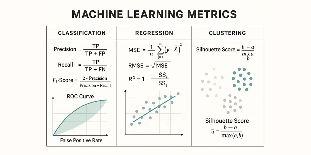
🧠 Classification Metrics

Used when the model predicts discrete labels (e.g., spam / not spam, disease / no disease). Let TP, FP, TN, FN represent the standard confusion matrix entries.

Metric	Description	Formula	Python Method
Accuracy	Measures the overall percentage of correct predictions. Best for balanced datasets.	\(Accuracy = \frac{TP + TN}{TP + TN + FP + FN}\)	accuracy_score(y_true, y_pred)
Precision	Out of all predicted positives, how many are actually positive. Useful when false positives are costly.	\(Precision = \frac{TP}{TP + FP}\)	precision_score(y_true, y_pred)
Recall (Sensitivity / TPR)	Out of all actual positives, how many did we correctly predict. Useful when missing positives is costly.	\(Recall = \frac{TP}{TP + FN}\)	recall_score(y_true, y_pred)
F1-Score	Harmonic mean of precision and recall — balances both.	\(F_1 = 2 \cdot \frac{Precision \cdot Recall}{Precision + Recall}\)	f1_score(y_true, y_pred)
Specificity (TNR)	Out of all actual negatives, how many were correctly predicted.	\(Specificity = \frac{TN}{TN + FP}\)	via confusion_matrix
ROC-AUC	Measures the model’s ability to distinguish classes. Closer to 1 = better.	Area under ROC curve	roc_auc_score(y_true, y_prob)
PR-AUC	Precision–Recall tradeoff, ideal for imbalanced datasets.	Area under PR curve	average_precision_score(y_true, y_prob)
Log Loss	Penalizes incorrect probabilities heavily. Ideal for probabilistic classifiers.	\(L = -\frac{1}{n}\sum [y_i\log(\hat{y}_i) + (1-y_i)\log(1-\hat{y}_i)]\)	log_loss(y_true, y_prob)

✅ Use:

• Precision when false positives are costly.
• Recall when false negatives are costly.
• F1 when balancing both is important.

🧩 Example: Classification Metrics

# Import common classification metrics
from sklearn.metrics import (
    accuracy_score,
    precision_score,
    recall_score,
    f1_score,
    roc_auc_score,
    average_precision_score,
    log_loss,
    confusion_matrix,
    classification_report
)

# Assume y_true are true labels and y_pred are predicted class labels
# y_prob are predicted probabilities (for ROC-AUC, PR-AUC, Log-Loss)
# Example:
# y_true = [0, 1, 1, 0, 1]
# y_pred = [0, 1, 0, 0, 1]
# y_prob = [0.1, 0.9, 0.4, 0.2, 0.8]

# ✅ Basic classification metrics
acc  = accuracy_score(y_true, y_pred)              # Overall correctness
prec = precision_score(y_true, y_pred)             # Positive predictive value
rec  = recall_score(y_true, y_pred)                # Sensitivity / True Positive Rate
f1   = f1_score(y_true, y_pred)                    # Balance between precision & recall

# ✅ Probabilistic metrics (for probabilistic classifiers)
roc_auc = roc_auc_score(y_true, y_prob)            # Area under ROC Curve
pr_auc  = average_precision_score(y_true, y_prob)  # Area under Precision-Recall Curve
logloss = log_loss(y_true, y_prob)                 # Penalizes wrong probability estimates

# ✅ Confusion Matrix (raw performance counts)
cm = confusion_matrix(y_true, y_pred)

# ✅ Detailed classification report (precision, recall, F1 per class)
report = classification_report(y_true, y_pred)

# Print results neatly
print(f"Accuracy       : {acc:.3f}")
print(f"Precision      : {prec:.3f}")
print(f"Recall         : {rec:.3f}")
print(f"F1 Score       : {f1:.3f}")
print(f"ROC-AUC        : {roc_auc:.3f}")
print(f"PR-AUC         : {pr_auc:.3f}")
print(f"Log Loss       : {logloss:.3f}")
print("\nConfusion Matrix:\n", cm)
print("\nClassification Report:\n", report)

⚙️ Tips:

• Accuracy → fraction of correct predictions overall.
• Precision → of all predicted positives, how many were correct.
• Recall → of all actual positives, how many were found.
• F1 Score → harmonic mean of precision and recall (balanced measure).
• ROC-AUC → model’s ability to separate classes.
• PR-AUC → preferred for imbalanced datasets (focuses on positive class).
• Log Loss → measures confidence of probability predictions (lower = better).
• Confusion Matrix → shows TP, FP, TN, FN counts — great for diagnostic insight.
• Classification Report → gives per-class Precision, Recall, F1, and Support.

🧠 Classification Metrics — Binary, Multi-Class & Multi-Label

✅ Use:

• Always use average='weighted' for imbalanced multi-class datasets.
• For multi-label tasks, average='micro' is preferred to capture global performance.
• Use classification_report() to summarize all metrics at once — it’s your go-to diagnostic summary.
• For probabilistic classifiers (like Logistic Regression, XGBoost, or Neural Nets), use y_prob to compute ROC-AUC, PR-AUC, or Log Loss.
• Always examine the confusion matrix — metrics may look good overall but hide class-specific issues.

🧩 Example: Classification Metrics — Binary, Multi-Class & Multi-Label

# -------------------------------------------------------------
# 🧠 IMPORTS
# -------------------------------------------------------------
from sklearn.metrics import (
    accuracy_score,
    precision_score,
    recall_score,
    f1_score,
    roc_auc_score,
    average_precision_score,
    log_loss,
    confusion_matrix,
    classification_report
)

# -------------------------------------------------------------
# 🧩 EXAMPLE DATA
# -------------------------------------------------------------
# Binary classification example
y_true_bin = [0, 1, 1, 0, 1]
y_pred_bin = [0, 1, 0, 0, 1]
y_prob_bin = [0.1, 0.9, 0.4, 0.2, 0.8]

# Multi-class example (3 classes)
y_true_multi = [0, 1, 2, 2, 1, 0]
y_pred_multi = [0, 2, 2, 1, 1, 0]
# For AUC-like metrics, you need probability estimates for each class (e.g., softmax output)
# y_prob_multi = model.predict_proba(X_test)

# Multi-label example (each sample can have multiple true labels)
y_true_multi_label = [
    [1, 0, 1],
    [0, 1, 0],
    [1, 1, 0],
]
y_pred_multi_label = [
    [1, 0, 1],
    [1, 1, 0],
    [0, 1, 0],
]

# -------------------------------------------------------------
# ✅ BINARY CLASSIFICATION METRICS
# -------------------------------------------------------------
print("=== Binary Classification Metrics ===")
acc_bin  = accuracy_score(y_true_bin, y_pred_bin)
prec_bin = precision_score(y_true_bin, y_pred_bin)
rec_bin  = recall_score(y_true_bin, y_pred_bin)
f1_bin   = f1_score(y_true_bin, y_pred_bin)
roc_bin  = roc_auc_score(y_true_bin, y_prob_bin)
pr_bin   = average_precision_score(y_true_bin, y_prob_bin)
logl_bin = log_loss(y_true_bin, y_prob_bin)
cm_bin   = confusion_matrix(y_true_bin, y_pred_bin)

print(f"Accuracy       : {acc_bin:.3f}")
print(f"Precision      : {prec_bin:.3f}")
print(f"Recall         : {rec_bin:.3f}")
print(f"F1 Score       : {f1_bin:.3f}")
print(f"ROC-AUC        : {roc_bin:.3f}")
print(f"PR-AUC         : {pr_bin:.3f}")
print(f"Log Loss       : {logl_bin:.3f}")
print("\nConfusion Matrix:\n", cm_bin)
print("\nClassification Report:\n", classification_report(y_true_bin, y_pred_bin))

# -------------------------------------------------------------
# ✅ MULTI-CLASS CLASSIFICATION METRICS
# -------------------------------------------------------------
print("\n=== Multi-Class Classification Metrics ===")

# average='macro' → treats all classes equally (useful when classes are balanced)
# average='weighted' → weights by support (better for imbalanced multi-class)
acc_multi  = accuracy_score(y_true_multi, y_pred_multi)
prec_macro = precision_score(y_true_multi, y_pred_multi, average='macro')
rec_macro  = recall_score(y_true_multi, y_pred_multi, average='macro')
f1_macro   = f1_score(y_true_multi, y_pred_multi, average='macro')
prec_weighted = precision_score(y_true_multi, y_pred_multi, average='weighted')
rec_weighted  = recall_score(y_true_multi, y_pred_multi, average='weighted')
f1_weighted   = f1_score(y_true_multi, y_pred_multi, average='weighted')

print(f"Accuracy (Overall)  : {acc_multi:.3f}")
print(f"Precision (Macro)   : {prec_macro:.3f}")
print(f"Recall (Macro)      : {rec_macro:.3f}")
print(f"F1 Score (Macro)    : {f1_macro:.3f}")
print(f"Precision (Weighted): {prec_weighted:.3f}")
print(f"Recall (Weighted)   : {rec_weighted:.3f}")
print(f"F1 Score (Weighted) : {f1_weighted:.3f}")
print("\nClassification Report:\n", classification_report(y_true_multi, y_pred_multi))

# -------------------------------------------------------------
# ✅ MULTI-LABEL CLASSIFICATION METRICS
# -------------------------------------------------------------
print("\n=== Multi-Label Classification Metrics ===")

# Here each label is evaluated independently; use averaging to aggregate
prec_micro = precision_score(y_true_multi_label, y_pred_multi_label, average='micro')
rec_micro  = recall_score(y_true_multi_label, y_pred_multi_label, average='micro')
f1_micro   = f1_score(y_true_multi_label, y_pred_multi_label, average='micro')

prec_samples = precision_score(y_true_multi_label, y_pred_multi_label, average='samples')
rec_samples  = recall_score(y_true_multi_label, y_pred_multi_label, average='samples')
f1_samples   = f1_score(y_true_multi_label, y_pred_multi_label, average='samples')

print(f"Precision (Micro) : {prec_micro:.3f}")
print(f"Recall (Micro)    : {rec_micro:.3f}")
print(f"F1 Score (Micro)  : {f1_micro:.3f}")
print(f"Precision (Samples): {prec_samples:.3f}")
print(f"Recall (Samples)   : {rec_samples:.3f}")
print(f"F1 Score (Samples) : {f1_samples:.3f}")
print("\nClassification Report:\n", classification_report(y_true_multi_label, y_pred_multi_label))

⚙️ Tips

Concept	Meaning	Common Usage
Binary Classification	Two classes (e.g., yes/no, 0/1).	Accuracy, F1, ROC-AUC, PR-AUC
Multi-Class	More than two classes (e.g., cat, dog, horse).	Macro- and Weighted- averages for F1, Precision, Recall
Multi-Label	Each sample can belong to multiple classes simultaneously.	Micro-average and sample-average metrics
Macro-Average	Treats each class equally (good for balanced datasets).	Gives equal weight to all classes.
Weighted-Average	Weighs metrics by class frequency.	Best for imbalanced data.
Micro-Average	Aggregates across all classes (global view).	Useful for multi-label or imbalanced setups.

---

📈 Regression Metrics

Used when predicting continuous values (e.g., house price, temperature, revenue).

Metric	Description	Formula	Python Method
MAE (Mean Absolute Error)	Average absolute difference between predicted and actual values. Easy to interpret.	\(MAE = \frac{1}{n}\sum | y_i - \hat{y}_i |\)	mean_absolute_error(y_true, y_pred)
MSE (Mean Squared Error)	Squares errors, penalizing large deviations. Sensitive to outliers.	\(MSE = \frac{1}{n}\sum (y_i - \hat{y}_i)^2\)	mean_squared_error(y_true, y_pred)
RMSE (Root Mean Squared Error)	Square root of MSE, same unit as the target.	\(RMSE = \sqrt{MSE}\)	mean_squared_error(y_true, y_pred, squared=False)
R² (Coefficient of Determination)	Proportion of variance in target explained by the model (1 = perfect).	\(R^2 = 1 - \frac{\sum (y_i - \hat y_i)^2}{\sum (y_i - \bar y)^2}\)	r2_score(y_true, y_pred)
MAPE (Mean Absolute Percentage Error)	Measures average percentage difference between prediction and actual. Easy to explain to non-tech users.	\(MAPE = \frac{100}{n}\sum \left | \frac{y_i - \hat{y}_i}{y_i}\right |\)	np.mean(np.abs((y_true - y_pred)/y_true))*100
SMAPE (Symmetric MAPE)	Handles zeros better by averaging actuals & predictions in denominator.	\(SMAPE = \frac{100}{n}\sum \frac{ | y_i - \hat{y}_i | }{( | y_i | + | \hat{y}_i | )/2}\)	2*np.mean(np.abs(y-y_hat)/(np.abs(y)+np.abs(y_hat)))*100

✅ Use:

• ✅ Use MAE or RMSE for general performance comparison.
• ✅ Prefer MAPE or SMAPE for percentage-based reporting (business metrics).
• ⚠️ Avoid MAPE when y_true contains zeros — use SMAPE instead.
• 💡 RMSLE is useful for targets with large magnitude variation (e.g., population, revenue).
• 📊 Use Adjusted R² for multi-feature models to account for model complexity.
• 🔍 Always visualize residuals to understand error distribution.

🧩 Example: Regression Metrics

# -------------------------------------------------------------
# 🧠 IMPORTS
# -------------------------------------------------------------
from sklearn.metrics import (
    mean_absolute_error,
    mean_squared_error,
    mean_absolute_percentage_error,
    median_absolute_error,
    r2_score,
    explained_variance_score
)
import numpy as np

# -------------------------------------------------------------
# 🧩 EXAMPLE DATA
# -------------------------------------------------------------
# Example: true vs predicted continuous values
# y_true = np.array([100, 200, 300, 400, 500])
# y_pred = np.array([110, 190, 310, 395, 480])

# -------------------------------------------------------------
# ✅ BASIC REGRESSION METRICS
# -------------------------------------------------------------

# Mean Absolute Error (MAE) → average absolute difference
mae = mean_absolute_error(y_true, y_pred)

# Mean Squared Error (MSE) → average of squared errors
mse = mean_squared_error(y_true, y_pred)

# Root Mean Squared Error (RMSE) → square root of MSE (same units as target)
rmse = mean_squared_error(y_true, y_pred, squared=False)

# R-squared (R²) → proportion of variance explained by model
r2 = r2_score(y_true, y_pred)

# Explained Variance Score → proportion of variance captured (less strict than R²)
evs = explained_variance_score(y_true, y_pred)

# -------------------------------------------------------------
# ✅ EXTENDED REGRESSION METRICS
# -------------------------------------------------------------

# Adjusted R-squared → adjusts R² for number of predictors (manual formula)
# n = number of observations, p = number of predictors
n, p = len(y_true), 1  # update 'p' as per number of features used
adj_r2 = 1 - ((1 - r2) * (n - 1) / (n - p - 1))

# Mean Absolute Percentage Error (MAPE) → avg. percentage error
# Built-in in sklearn >= 0.24
try:
    mape = mean_absolute_percentage_error(y_true, y_pred) * 100
except:
    mape = np.mean(np.abs((y_true - y_pred) / y_true)) * 100

# Symmetric Mean Absolute Percentage Error (SMAPE) → bounded [0–200]%
smape = 100 * np.mean(
    2 * np.abs(y_true - y_pred) / (np.abs(y_true) + np.abs(y_pred))
)

# Root Mean Squared Log Error (RMSLE) → penalizes underestimation
rmsle = np.sqrt(mean_squared_error(np.log1p(y_true), np.log1p(y_pred)))

# Median Absolute Error (MedAE) → robust to outliers
medae = median_absolute_error(y_true, y_pred)

# -------------------------------------------------------------
# ✅ PRINT RESULTS NEATLY
# -------------------------------------------------------------
print(f"Mean Absolute Error (MAE)        : {mae:.3f}")
print(f"Mean Squared Error (MSE)         : {mse:.3f}")
print(f"Root Mean Squared Error (RMSE)   : {rmse:.3f}")
print(f"R-squared (R²)                   : {r2:.3f}")
print(f"Adjusted R-squared (Adj R²)      : {adj_r2:.3f}")
print(f"Explained Variance Score (EVS)   : {evs:.3f}")
print(f"Mean Absolute % Error (MAPE)     : {mape:.3f}%")
print(f"Symmetric MAPE (SMAPE)           : {smape:.3f}%")
print(f"Root Mean Squared Log Error      : {rmsle:.3f}")
print(f"Median Absolute Error (MedAE)    : {medae:.3f}")

---

⚙️ Tips:

Metric	Meaning	Notes
MAE	Average of absolute errors	Easy to interpret; robust to outliers.
MSE	Average of squared errors	Penalizes large deviations more.
RMSE	Square root of MSE	Same scale as original data.
R² (Coefficient of Determination)	Proportion of variance explained	1 = perfect fit, 0 = poor fit.
Adjusted R²	R² adjusted for #features	Prevents artificial inflation with many predictors.
EVS (Explained Variance Score)	Variation captured by model	Similar to R² but less strict.
MAPE	Avg. percentage error	Interpretable in %. Avoid if y_true has zeros.
SMAPE	Symmetric version of MAPE	Bounded (0–200%), handles zeros better.
RMSLE	Penalizes underestimation	Useful when target values vary exponentially.
MedAE	Median of absolute errors	Robust alternative to MAE for skewed data.

---

📦 Clustering Metrics (Unsupervised)

These metrics measure the compactness and separation of clusters.

Metric	Description	Formula / Idea	Python Method
Silhouette Score	How close each point is to its own cluster vs. others (−1 to +1). Higher = better.	\(s = \frac{b - a}{\max(a,b)}\) where a = intra-cluster, b = nearest cluster distance.	silhouette_score(X, labels)
Silhouette Samples	Per-sample silhouette values — useful to diagnose which points are poorly clustered.	Same as above, returned per sample (s_i).	sklearn.metrics.silhouette_samples(X, labels)
Calinski-Harabasz Index (CH)	Ratio of between-cluster dispersion to within-cluster dispersion. Higher = better (more separated, compact clusters).	\(CH = \frac{\text{trace}(B_k)/(k-1)}{\text{trace}(W_k)/(n-k)}\) where (B_k) between-group dispersion, (W_k) within-group.	calinski_harabasz_score(X, labels)
Davies–Bouldin Index (DBI)	Average similarity between each cluster and its most similar one. Lower = better (compact, well-separated clusters).	For cluster i with scatter (s_i) and centroid distance (d_{ij}): \(DB = \frac{1}{k}\sum_i \max_{j\ne i}\frac{s_i + s_j}{d_{ij}}\)	davies_bouldin_score(X, labels)
Adjusted Rand Index (ARI)	Measures similarity between predicted clusters and ground-truth labels, corrected for chance. 1 = perfect agreement, ~0 = random.	Based on pair counting (agreements vs disagreements), adjusted for expected index. (See ARI definition in literature.)	adjusted_rand_score(true_labels, pred_labels)
Rand Index (RI)	Fraction of label pairs on which clusterings agree (does not correct for chance).	RI = (number of agreement pairs) / (total pairs).	rand_score(true_labels, pred_labels) (newer sklearn) or compute from confusion matrix.
Normalized Mutual Information (NMI)	Measures shared information between cluster assignment and true labels, normalized to [0,1]. Higher = better.	\(NMI(U,V)=\frac{I(U;V)}{\sqrt{H(U)H(V)}}\) where (I) = mutual information, (H)=entropy.	normalized_mutual_info_score(true_labels, pred_labels)
Mutual Information (MI)	Raw mutual information between clustering and labels (not normalized).	(I(U;V)=\sum_{u,v} p(u,v)\log\frac{p(u,v)}{p(u)p(v)})	mutual_info_score(true_labels, pred_labels)
Adjusted Mutual Info (AMI)	Mutual information adjusted for chance. Like ARI but information-theoretic.	Adjusts MI by expected MI under random labeling.	adjusted_mutual_info_score(true_labels, pred_labels)
Homogeneity	Each cluster contains only members of a single class (pure clusters). Range 0..1.	Homogeneity = 1 when each cluster has single class. Related to conditional entropy H(Class	Cluster).	homogeneity_score(true_labels, pred_labels)
Completeness	All members of a given class are assigned to the same cluster. Range 0..1.	Related to H(Cluster | Class).	completeness_score(true_labels, pred_labels)
V-measure	Harmonic mean of Homogeneity and Completeness (balanced). Range 0..1.	\(V = 2\cdot\frac{\text{homogeneity}\cdot\text{completeness}}{\text{homogeneity}+\text{completeness}}\)	v_measure_score(true_labels, pred_labels)
Fowlkes–Mallows Index (FMI)	Geometric mean of precision and recall over pairs (pairwise precision/recall). Higher = better.	\(FMI = \sqrt{\frac{TP}{TP+FP}\cdot\frac{TP}{TP+FN}}\) where TP/FP/FN are pair counts.	fowlkes_mallows_score(true_labels, pred_labels)
Purity	Simple external metric: fraction of cluster members that belong to the majority true class in that cluster. Easy to interpret but not normalized.	\(Purity = \frac{1}{n}\sum_i \max_j |C_i \cap T_j|\) where $C_i$ cluster, $T_j$ true class.	Not in sklearn by default — compute from contingency matrix (sklearn.metrics.cluster.contingency_matrix) then apply formula.
Jaccard Index (pairwise)	Pairwise similarity: intersection over union of pair assignments. Useful for comparing clusterings.	For sets A,B: \(\(J(A,B)=\frac{ | A\cap B | }{ | A\cup B | }\)\). For clustering, use pairwise version.	sklearn.metrics.jaccard_score for binary; cluster-level custom computation or sklearn.metrics.pairwise_distances / contingency-based code.
Noise Ratio (DBSCAN)	Fraction of points labeled as noise (-1) by DBSCAN. Lower noise ratio usually preferred (but depends on task).	\(\text{noise ratio} = \frac{\text{count\(labels = -1\)}}{n}\)	Compute from labels array: np.mean(labels == -1)
Dunn Index	Measures cluster separation / compactness (higher = better). Sensitive to outliers; not in sklearn.	\(D = \frac{\min_{i\ne j} \delta(C_i,C_j)}{\max_k \Delta(C_k)}\) where (\delta) inter-cluster distance, (\Delta) intra-cluster diameter.	Not in sklearn — custom implementation required (use pairwise distances).

✅ Use:

• Use internal metrics (silhouette, CH, DBI) when you do not have ground-truth labels. They measure compactness and separation.
• Use external metrics (ARI, NMI) when you do have reliable true labels for validation. They compare clustering to a known truth.
• For DBSCAN, check -1 labels (noise); internal metrics may be undefined if too few clusters exist.

• Always visualize clusters (scatter, PCA, t-SNE) alongside metrics — numbers alone can be misleading.

• Silhouette Samples help find misclustered points — useful for visualization and debugging.
• Purity is easy to explain to stakeholders but can be biased by many small clusters — pair with other metrics.
• Some metrics aren’t in sklearn (Purity, Dunn): compute from contingency / distance matrices if needed.

🧩 Example: Clustering Metrics

# -------------------------------------------------------------
# Imports
# -------------------------------------------------------------
import numpy as np
from sklearn.datasets import make_blobs
from sklearn.cluster import KMeans, DBSCAN
from sklearn.metrics import (
    silhouette_score,
    silhouette_samples,
    calinski_harabasz_score,
    davies_bouldin_score,
    adjusted_rand_score,
    normalized_mutual_info_score,
    homogeneity_score,
    completeness_score,
    v_measure_score,
)

# -------------------------------------------------------------
# Example data (synthetic) and clustering
# -------------------------------------------------------------
X, y_true = make_blobs(n_samples=500, centers=4, cluster_std=0.60, random_state=42)

# KMeans clustering (example)
n_clusters = 4
kmeans = KMeans(n_clusters=n_clusters, random_state=42)
labels_km = kmeans.fit_predict(X)

# DBSCAN clustering (density-based example)
db = DBSCAN(eps=0.6, min_samples=5)
labels_db = db.fit_predict(X)  # -1 indicates noise in DBSCAN

# -------------------------------------------------------------
# Internal / Unsupervised Metrics (no ground-truth required)
# -------------------------------------------------------------
# Silhouette Score (range -1..1): higher is better; requires >=2 clusters
sil_score_km = silhouette_score(X, labels_km)              # KMeans
sil_score_db = silhouette_score(X, labels_db) if len(set(labels_db)) > 1 else float('nan')

# Silhouette values per sample (useful for diagnostics)
sil_samples = silhouette_samples(X, labels_km)

# Calinski-Harabasz Index: higher is better (between-cluster / within-cluster)
ch_score_km = calinski_harabasz_score(X, labels_km)

# Davies-Bouldin Index: lower is better (compactness vs separation)
db_index_km = davies_bouldin_score(X, labels_km)

# -------------------------------------------------------------
# External / Labelled Metrics (require ground-truth labels)
# -------------------------------------------------------------
# Adjusted Rand Index (ARI): 1=perfect agreement, ~0 random
ari_km = adjusted_rand_score(y_true, labels_km)

# Normalized Mutual Information (NMI): 0..1, higher better
nmi_km = normalized_mutual_info_score(y_true, labels_km)

# Homogeneity, Completeness, V-measure
homog = homogeneity_score(y_true, labels_km)
compl = completeness_score(y_true, labels_km)
vmes = v_measure_score(y_true, labels_km)

# -------------------------------------------------------------
# Print results
# -------------------------------------------------------------
print("=== KMeans clustering metrics ===")
print(f"Number of clusters (KMeans)        : {len(set(labels_km))}")
print(f"Silhouette Score (KMeans)          : {sil_score_km:.4f}")
print(f"Calinski-Harabasz Index (KMeans)   : {ch_score_km:.4f}")
print(f"Davies-Bouldin Index (KMeans)     : {db_index_km:.4f}")
print(f"Adjusted Rand Index (KMeans)       : {ari_km:.4f}")
print(f"NMI (KMeans)                       : {nmi_km:.4f}")
print(f"Homogeneity                         : {homog:.4f}")
print(f"Completeness                        : {compl:.4f}")
print(f"V-measure                           : {vmes:.4f}")

print("\n=== DBSCAN clustering metrics ===")
n_clusters_db = len(set(labels_db)) - (1 if -1 in labels_db else 0)
print(f"Estimated clusters (DBSCAN)         : {n_clusters_db} (noise points labeled -1)")
if np.isfinite(sil_score_db):
    print(f"Silhouette Score (DBSCAN)          : {sil_score_db:.4f}")
else:
    print("Silhouette Score (DBSCAN)          : N/A (need >=2 labelled clusters)")

# -------------------------------------------------------------
# Optional: quick diagnostic summaries
# -------------------------------------------------------------
# Proportion of noise for DBSCAN
noise_ratio = np.mean(np.array(labels_db) == -1)
print(f"DBSCAN noise ratio                  : {noise_ratio:.3f}")

⚙️ Tips:

• Silhouette Score: how similar a point is to its own cluster vs the nearest other cluster. Values near +1 mean well-clustered; near -1 mean misclassified.
• Silhouette Samples: per-sample scores useful for plotting/diagnostics (e.g., identify bad clusters).
• Calinski–Harabasz: ratio of between-cluster dispersion to within-cluster dispersion — larger is better.
• Davies–Bouldin: average similarity between each cluster and its most similar one — smaller is better.
• Adjusted Rand Index (ARI): compares clusters to ground-truth labels (corrects for chance).
• Normalized Mutual Information (NMI): measures shared information between clustering and true labels.
• Homogeneity / Completeness / V-measure: explain how pure clusters are (homogeneity) and how complete true classes are captured (completeness); v-measure = harmonic mean.

---

🔍 Ranking / Recommendation Metrics

Used for recommendation systems, search ranking, or top-k predictions. Ranking and recommendation systems evaluate how well a model orders or recommends items based on relevance or preference.

Unlike classification, which predicts what, ranking cares about how high relevant results appear.

Metric	Description	Formula / Concept	Python Method
Precision@k	Fraction of top-k recommended items that are relevant.	\(P@k = \frac{\text{Relevant items in top }k}{k}\)	Custom function
Recall@k	Fraction of total relevant items retrieved in top-k list.	\(R@k = \frac{\text{Relevant items in top }k}{\text{Total relevant items}}\)	Custom function
MAP (Mean Average Precision)	Average of precision values across recall levels. Higher = better ranking.	\(MAP = \frac{1}{Q}\sum_q AvgPrecision(q)\)	average_precision_score()
NDCG (Normalized Discounted Cumulative Gain)	Measures ranking quality considering order and relevance.	\(NDCG@k = \frac{DCG@k}{IDCG@k}\)	ndcg_score(y_true, y_score)

✅ Use:

• Search Engines: rank documents by query relevance (Google, Bing).
• Recommender Systems: suggest products, movies, or news items (Amazon, Netflix).
• Information Retrieval (IR): evaluate top-k precision and recall.

• Personalization Systems: adapt ranking to user profiles and click history.

• Precision@k: Measures short-term relevance — good for search and top-N recommendation quality.

• Recall@k: Focuses on coverage — how much of what user wants appears in top-k.
• MAP (Mean Average Precision): Combines ranking accuracy and completeness — robust for IR and recommendation.
• MRR (Mean Reciprocal Rank): Average reciprocal of the rank of the first relevant item. Prioritizes early relevance — ideal for Q&A or retrieval systems.
• NDCG (Normalized Discounted Cumulative Gain): Handles graded relevance; common in search engines. Weighted ranking quality — higher relevance at higher ranks yields more gain.
• Hit Rate (HR@k): Binary form of recall@k — easier to interpret. Whether at least one relevant item appears in top-k.
• Coverage: Reflects diversity — higher coverage = model recommends wider variety. Fraction of all items ever recommended to any user.
• Diversity: Encourages variety; avoids echo chambers or repetitive results. Average dissimilarity between recommended items.
• Novelty: Ensures recommendations surface less-seen items. Popularity bias measure — lower popularity → higher novelty.
• Serendipity: Enhances user satisfaction beyond predictability. Measures how surprising but relevant the recommendation is.

🧩 Example

import numpy as np
from sklearn.metrics import ndcg_score, average_precision_score

# Example: relevance scores for each query (user)
y_true = np.asarray([[3, 2, 3, 0, 1, 2]])   # true relevance grades
y_score = np.asarray([[0.8, 0.3, 0.7, 0.1, 0.2, 0.4]])  # predicted scores

# NDCG (Normalized Discounted Cumulative Gain) @ K=5
ndcg = ndcg_score(y_true, y_score, k=5)
print(f"NDCG@5: {ndcg:.3f}")

# MAP (Mean Average Precision)
map_score = average_precision_score((y_true > 0).ravel(), y_score.ravel())
print(f"MAP: {map_score:.3f}")

⚙️ Tips:

When / Goal	Preferred Metric(s)	Tips & Insights
You want the top-k results to be correct.	Precision@k, NDCG, Hit Rate	Tune for higher precision; good for homepage or top-N recommendations.
You care about retrieving all relevant items.	Recall@k, MAP	Important for archival search, playlist or content retrieval.
You want early relevant results.	MRR, NDCG	Ideal for search ranking and question answering (QA).
You want balanced ranking quality.	MAP, NDCG	Use for general ranking system evaluation.
You want model diversity / user satisfaction.	Coverage, Diversity, Novelty, Serendipity	Add as secondary optimization targets to avoid redundancy.
You have implicit feedback only (clicks/views).	Hit Rate, NDCG	Suitable when explicit “relevance” labels aren’t available.

💡 Practical Takeaways

• Ranking metrics depend on order, not absolute scores — focus on relative correctness.
• Precision@k and Recall@k are easy to compute but ignore graded relevance — prefer NDCG when relevance is multi-level (e.g., 0–3 scale).
• MAP provides a single global score combining precision and recall — excellent for comparing models.
• MRR emphasizes how quickly the first relevant item appears — good for retrieval.
• Track Diversity, Coverage, and Novelty to ensure real-world user satisfaction and system robustness.
• Always evaluate both offline (metrics) and online (A/B tests, click-through rates).

TODO

5. Practical Python Snippets

🧩 Logistic Regression (Scikit-Learn)

from sklearn.model_selection import train_test_split
from sklearn.preprocessing import StandardScaler
from sklearn.linear_model import LogisticRegression
from sklearn.metrics import classification_report

# Split and scale
X_train, X_test, y_train, y_test = train_test_split(X, y, test_size=0.2, random_state=42)
scaler = StandardScaler()
X_train = scaler.fit_transform(X_train)
X_test = scaler.transform(X_test)

# Train
model = LogisticRegression(max_iter=1000)
model.fit(X_train, y_train)
print(classification_report(y_test, model.predict(X_test)))

🧠 Minimal PyTorch Network

import torch
from torch import nn

class SimpleNet(nn.Module):
    def __init__(self, in_dim):
        super().__init__()
        self.layers = nn.Sequential(
            nn.Linear(in_dim, 64),
            nn.ReLU(),
            nn.Linear(64, 32),
            nn.ReLU(),
            nn.Linear(32, 1)
        )
    def forward(self, x):
        return self.layers(x)

model = SimpleNet(X.shape[1])
criterion = nn.MSELoss()
optimizer = torch.optim.Adam(model.parameters(), lr=1e-3)

---

6. Best Practices & Common Pitfalls

✅ Best Practices	⚠️ Common Pitfalls
Start simple, add complexity only when justified	Data leakage (using target info in features)
Use proper cross-validation	Ignoring feature scaling for ML models
Track experiments & reproducibility	Overfitting small datasets
Align metrics with business goals	Over-reliance on accuracy
Monitor deployed model drift	Poor validation strategy (esp. time series)

---

7. Quick Comparison Tables

🔸 ML vs DL

Aspect	Machine Learning	Deep Learning
Data Requirement	Low–Medium	High
Feature Engineering	Manual	Automatic
Interpretability	High	Low
Compute Demand	Low	High
Use Cases	Tabular data, small samples	Images, text, large-scale tasks

---

8. Deployment Checklist

• ✅ Save trained model artifact with metadata
• ✅ Validate input schema & pipeline consistency
• ✅ Monitor performance & data drift
• ✅ Automate retraining or alerts
• ✅ Secure access and governance

---

9. Analogy & Plain Explanation

• Machine Learning: like teaching a student with examples and grading them.
• Deep Learning: like a student discovering sub-skills automatically (edges → shapes → objects).
• Metrics: your grading system — tells you if the student is learning correctly.

---

10. Quick Upgrade Path

1. Study transformers and attention mechanisms
2. Learn MLOps: CI/CD, feature stores, versioning
3. Explore Explainable AI (SHAP, LIME)
4. Implement ethical AI and bias mitigation
5. Practice with real projects — Kaggle, open datasets

---

📊 DSML Metrics — Comprehensive Guide ✅

CCC

⏱️ 5. Time Series / Forecasting Metrics

Used when predicting values over time (sales, temperature, stock prices). Emphasis on directional accuracy and scale-independent errors.

Metric	Description	Formula	Python Method
MAE	Average of absolute errors; robust and easy to interpret.	\(MAE = \frac{1}{n}\sum | y_t - \hat y_t |\)	mean_absolute_error(y_true, y_pred)
RMSE	Penalises larger errors; sensitive to outliers.	\(RMSE = \sqrt{\frac{1}{n}\sum (y_t - \hat y_t)^2}\)	mean_squared_error(y_true, y_pred, squared=False)
MAPE	Average percentage error; intuitive but unstable for near-zero values.	\(MAPE = \frac{100}{n}\sum \left | \frac{y_t - \hat y_t}{y_t}\right |\)	np.mean(np.abs((y_true - y_pred)/y_true))*100
SMAPE	Symmetric version of MAPE; bounded between 0–200%.	\(SMAPE = \frac{100}{n}\sum \frac{ | y_t - \hat y_t | }{( | y_t | + | \hat y_t | )/2}\)	Custom NumPy formula
RMSPE	Root mean square percentage error; scale-free measure.	\(RMSPE = 100 \sqrt{\frac{1}{n}\sum \left(\frac{y_t - \hat y_t}{y_t}\right)^2}\)	Custom NumPy formula

---

🧭 6. Summary: Choosing the Right Metric

Problem Type	Typical Metrics	Use When
Classification	Accuracy, F1, ROC-AUC	Balanced or imbalanced label prediction
Regression	MAE, RMSE, R², MAPE	Predicting continuous targets
Clustering	Silhouette, CH, DBI	Evaluating cluster quality
Ranking / Recommender	MAP, NDCG, Precision@k	Personalized recommendations, search
Forecasting	MAPE, SMAPE, RMSE	Time series or sequential predictions

---

🧭 7. Key Takeaways

• Always choose a metric aligned with your business goal. (e.g., Recall for fraud detection, MAPE for forecast accuracy).
• Use cross-validation for robust metric estimation.
• Track multiple metrics — one metric rarely tells the full story.
• In production, monitor metrics drift to detect model decay.

---

⚙️ Notes & Tips

• Scikit-learn: Choosing the right estimator
• Supervised Learning dominates applied ML (most business problems have labeled data).
• Unsupervised Learning is used for discovery, not prediction.
• Semi/Self-Supervised Learning bridges gaps where labeled data is scarce.
• Reinforcement Learning is powerful but data-hungry and environment-dependent.
• Deep Learning cuts across all categories — when data is large and complex.
• Always align metrics with your business objective (precision for spam filters, recall for disease detection, MAPE for forecasts).

---

🧩 Plain-Language Summary for Beginners

Category	Plain Meaning	What It Learns	Example
Supervised Learning	Learns from examples with correct answers (labeled data).	Input → Output mapping.	Predicting loan default, image classification.
Unsupervised Learning	Learns from unlabeled data to find hidden patterns.	Data structure or clusters.	Grouping customers by purchase behavior.
Semi-Supervised Learning	Learns from a few labeled + many unlabeled examples.	Extends labeled data usefulness.	Medical image analysis (few labeled scans).
Self-Supervised Learning	Creates labels automatically from raw data.	Learns general representations.	Predict masked words in sentences (BERT).
Reinforcement Learning	Learns through trial and error to maximize reward.	Policy or strategy.	Self-driving cars, game agents.
Deep Learning	Uses large neural networks to learn features automatically.	Complex feature hierarchies.	Face recognition, speech translation.

---

✅ Simplified View (At a Glance)

ML Category	Typical Problems	Typical Metrics	Example Use-Case
Supervised Learning (SL)	Classification, Regression	Accuracy, F1, ROC-AUC, MAE, RMSE	Spam detection, price prediction
Unsupervised Learning (USL)	Clustering, Dimensionality Reduction	Silhouette, CH, DBI, Explained Variance	Customer segmentation, visualization
Semi-Supervised Learning (SSL)	Hybrid labeled/unlabeled learning	Accuracy, F1, ROC-AUC	Learning from few labeled samples
Self-Supervised Learning (Self-SL)	Pretext predictive tasks	Representation quality, Transfer Accuracy	Pretraining models on unlabeled data
Reinforcement Learning (RL)	Sequential decision-making	Reward, Cumulative Return	Robotics, games, trading bots
Deep Learning (DL)	Vision, NLP, Audio, Generative tasks	Accuracy, IoU, BLEU, FID	Image, speech, and text understanding
Forecasting / Time-Series	Predicting future trends	MAPE, SMAPE, RMSE	Sales, weather, demand forecasts
Ranking / Recommendation	Search / recommender systems	Precision@k, Recall@k, NDCG	Netflix, YouTube, Google Search
Anomaly Detection	Rare-event detection	F1, ROC-AUC, PR-AUC	Fraud, defect detection

---

🧭 ML Categories, Problem Type & Evaluation Metrics

ML Category	Problem Type	Sub-Category / Nature	Typical Metrics	Use When / Description
Supervised Learning (SL)	Classification	Binary / Multi-class / Multi-label / Imbalanced	Accuracy, Precision, Recall, F1-Score, ROC-AUC, PR-AUC, Log-Loss	When you have labeled data (known outputs). The model learns to map input → output. Example: spam detection, disease diagnosis.
	Regression	Linear / Nonlinear / Robust / Percentage-based	MAE, MSE, RMSE, R², MAPE, SMAPE	When predicting continuous values (e.g., prices, temperature). MAPE and SMAPE express accuracy as % error.
Unsupervised Learning (USL)	Clustering	Partition-based, Hierarchical, Density-based	Silhouette Score, Calinski-Harabasz Index, Davies-Bouldin Index	When no labels exist; model groups similar data. Example: customer segmentation.
	Dimensionality Reduction	PCA, t-SNE, UMAP	Reconstruction Error, Explained Variance	When simplifying features while preserving structure. Example: visualization, compression.
Semi-Supervised Learning (SSL)	Hybrid Tasks	Few labeled + many unlabeled samples	Accuracy, F1-Score, Log-Loss, ROC-AUC (on labeled subset)	When labeled data is expensive or scarce. Example: labeling a few medical images, learning from rest automatically.
Self-Supervised Learning (Self-SL)	Representation Learning	Contrastive, Masked Prediction, Autoencoding	Pretext-task accuracy, Transfer Learning performance	Model generates pseudo-labels from data itself. Example: predicting masked words in text (BERT), missing pixels in images.
Reinforcement Learning (RL)	Decision / Control Tasks	Single-agent / Multi-agent / Continuous / Discrete	Reward, Cumulative Return, Average Reward, Success Rate	Model learns by interacting with environment via trial-and-error. Example: robotics, game AI.
Deep Learning (DL)	Supervised DL	CNNs (images), RNNs (sequences), Transformers (text)	Accuracy, F1-Score, IoU, BLEU, ROUGE	Applies neural networks to complex data. Example: image classification, translation, text summarization.
	Unsupervised DL	Autoencoders, GANs, VAEs	Reconstruction Loss, FID, Inception Score	Learns structure or generates new samples without labels. Example: synthetic image generation.
	Self-Supervised DL	Pretraining models using pseudo-tasks	Linear Probe Accuracy, Fine-tune Accuracy	Foundation models trained on large unlabeled corpora; adapted to downstream tasks.
Specialized Domains (Cross-Cutting)	Ranking / Recommender Systems	Search, Recommendation, Personalization	Precision@k, Recall@k, MAP, NDCG	Measures top-k relevance and ordering of results. Example: Netflix, Google Search.
	Forecasting (Time-Series)	Univariate / Multivariate / Multi-step	MAPE, SMAPE, RMSE, MAE	Predicts future values from past data. Example: sales, demand, energy load.
	Anomaly Detection	Supervised / Unsupervised	Precision@k, Recall@k, F1, ROC-AUC, PR-AUC	Detects rare abnormal events. Example: fraud, system failures.
	Natural Language Processing (NLP)	Text Classification / NER / Translation	Accuracy, F1, BLEU, ROUGE, METEOR	Evaluates language model outputs. Example: sentiment analysis, summarization.
	Computer Vision (CV)	Object Detection / Segmentation / Recognition	mAP, IoU, Dice, Pixel Accuracy	Measures visual recognition accuracy. Example: detecting cars or faces in images.
	Generative Models	GANs, Diffusion Models	FID, Inception Score, Perplexity	Evaluates realism and diversity of generated outputs. Example: image or text synthesis.

---

📚 References

• Validated from official documentation, academic repositories, and industry sources.
• Recommended reading flow:
  → Foundations → Evaluation Metrics → Paradigms → Practical Guides.
• Combine conceptual (Wikipedia, IBM, MIT) with applied (scikit-learn, Google MLCC) for holistic mastery.

🧠 Core Machine Learning Foundations

1. Machine Learning — Wikipedia
2. What Is Machine Learning — IBM Think
3. Machine Learning Overview — GeeksforGeeks
4. Introduction to Machine Learning — GeeksforGeeks
5. Machine Learning Explained — MIT Sloan

⚙️ Evaluation & Metrics (Classification, Regression, Clustering, Ranking)

1. Scikit-Learn: Model Evaluation — Official Docs
2. Scikit-Learn — Ranking Metrics
3. Google ML Crash Course — Classification & Metrics
4. Google ML Crash Course — Regression Metrics
5. Google ML — Recommendation System Evaluation
6. Papers With Code — Evaluation Metrics by Domain
7. Precision and Recall — Wikipedia
8. Mean Absolute Percentage Error (MAPE) — Wikipedia
9. Coefficient of Determination (R²) — Wikipedia
10. Information Retrieval — Evaluation (Wikipedia)

🔍 Specialized Learning Paradigms

1. Reinforcement Learning — Wikipedia
2. Self-Supervised Learning — Wikipedia
3. Deep Learning — Wikipedia

🧩 Supplementary & Practical Guides

1. Regression Models in ML — GeeksforGeeks
2. Machine Learning Algorithms — IBM Think

---