🧭 DSML: Machine Learning Lifecycle - Comprehensive Guide
Concise, clear, and validated Comprehesive guide revision notes on Machine Learning Lifecycle, MLOps, Metrics, Code Snippets — structured for beginners and practitioners.
Introduction
The Machine Learning Lifecycle is a structured, iterative framework that guides the complete development, deployment, and maintenance of machine learning systems. It provides a systematic methodology for transforming business problems into operational AI solutions that deliver sustained value. Unlike traditional software development, the ML lifecycle emphasizes continuous improvement, data centricity, and adaptive model management throughout the entire project duration.
The lifecycle is fundamentally cyclical and iterative rather than linear—models are never truly “finished” but require ongoing refinement, retraining, and optimization based on real-world performance, evolving data patterns, and changing business requirements.
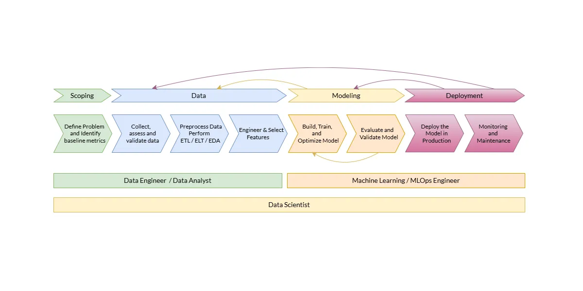 Machine Learning Lifecycle Illustrated
Key Characteristics
- Iterative Nature: Phases are revisited multiple times based on insights gained in subsequent stages
- Data-Centric: Quality, quantity, and representativeness of data directly determine model performance
- Quality Assurance: Each phase incorporates validation checkpoints and risk mitigation strategies
- Cross-Functional Collaboration: Requires coordination between data scientists, engineers, domain experts, and business stakeholders
- Continuous Process: Post-deployment monitoring and maintenance are integral, not optional components
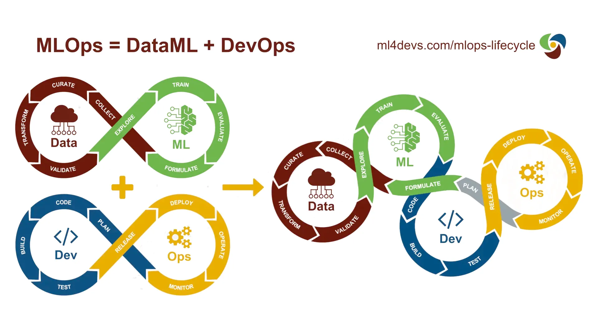
Lifecycle Terminology: Comparative Analysis
Different organizations, frameworks, and practitioners use varying terminology to describe ML lifecycle phases. Understanding these equivalences is crucial for cross-team communication and literature comprehension.
Table 1: Phase Terminology Across Major Frameworks
| Generic Phase | CRISP-DM (1999) | CRISP-ML(Q) (2020) | MLOps/AWS | OSEMN | SEMMA | Team DataScience | Academic/Research |
|---|---|---|---|---|---|---|---|
| Business Understanding | Business Understanding | Business & Data Understanding | Business Problem Framing | - | - | Scoping | Problem Definition |
| Data Acquisition | Data Understanding | Data Understanding | Data Processing | Obtain | Sample | Data | Data Collection |
| Data Preparation | Data Preparation | Data Preparation | Data Processing | Scrub | Explore | Data Engineering | Data Preprocessing |
| Exploratory Analysis | Data Understanding | Data Understanding | Data Processing | Explore | Explore | Data Engineering | EDA |
| Feature Engineering | Data Preparation | Data Preparation | Data Processing | - | Modify | Data Engineering | Feature Engineering |
| Model Development | Modeling | Modeling | Model Development | Model | Model | Model Engineering | Model Building |
| Model Training | Modeling | Modeling | Model Development | Model | Model | Model Engineering | Training |
| Model Evaluation | Evaluation | Evaluation | Model Development | iNterpret | - | Model Engineering | Validation/Testing |
| Deployment | Deployment | Deployment | Deployment | - | - | Deployment | Productionization |
| Monitoring | - | Monitoring & Maintenance | Monitoring | - | - | Deployment | Post-Deployment |
Table 2: Hierarchical Terminology Structure
| Hierarchy Level | Category Name | Subcategories | Granularity | Time Allocation (%) |
|---|---|---|---|---|
| Level 1: Macro | Project Lifecycle | Experimental Phase, Production Phase | Project-wide phases spanning weeks-months | 100% |
| Level 2: Meso | Major Phases | Business & Data, Modeling, Operations | Distinct functional areas | 30% / 50% / 20% |
| Level 3: Micro | Specific Stages | Problem Definition → Collection → Cleaning → EDA → Feature Engineering → Selection → Training → Evaluation → Tuning → Deployment → Monitoring → Maintenance | Sequential workflow steps | 5-15% each |
| Level 4: Granular | Technical Tasks | Imputation, encoding, normalization, cross-validation, hyperparameter tuning, A/B testing, drift detection | Individual technical operations | 1-5% each |
| Level 5: Atomic | Code-Level Operations | Function calls, API requests, data transformations, metric calculations | Implementation details | < 1% each |
Table 3: Terminology Equivalence Matrix
| Context/Source | Phase 1 | Phase 2 | Phase 3 | Phase 4 | Phase 5 | Phase 6 | Phase 7 |
|---|---|---|---|---|---|---|---|
| Industry Standard | Problem Framing | Data Engineering | Model Engineering | Evaluation | Deployment | Monitoring | Maintenance |
| Academic | Problem Definition | Data Collection | Model Development | Validation | Implementation | Performance Tracking | Optimization |
| Business-Oriented | Business Case | Data Acquisition | Solution Building | Testing | Go-Live | Performance Management | Continuous Improvement |
| Technical | Scoping | ETL Pipeline | Algorithm Selection & Training | Metrics Assessment | Production Deployment | Observability | Retraining |
| Agile ML | Sprint 0 Planning | Data Sprint | Model Sprint | Validation Sprint | Release Sprint | Monitor Sprint | Iterate Sprint |
Phase-by-Phase Comprehensive Breakdown
Phase 1: Business & Problem Understanding
Objective: Establish clear comprehension of the business problem and translate it into a tractable machine learning task with defined success criteria.
Key Activities
1.1 Business Context Analysis
- Identify core business problem requiring solution
- Understand organizational goals, constraints, and strategic alignment
- Assess stakeholder expectations and requirements
- Analyze current processes and pain points
- Determine competitive landscape and market dynamics
1.2 Problem Statement Formulation
- Define clear, specific, and measurable objectives
- Translate business metrics into machine learning metrics
- Example: “Reduce customer churn by 15%” → “Predict churn probability with 80% recall and 65% precision”
- Specify project scope, boundaries, and limitations
- Establish both business and technical success criteria
- Define what constitutes project failure or success
1.3 Feasibility Assessment
Critical questions to address:
| Dimension | Key Questions | Risk Mitigation |
|---|---|---|
| Data Availability | Do we have sufficient quality data? Can we obtain it? | Conduct data inventory, explore external sources, consider synthetic data |
| ML Applicability | Is ML the right solution? Could simpler methods work? | Benchmark against rule-based systems, calculate complexity-benefit ratio |
| Technical Feasibility | Do we have necessary infrastructure? Can we scale? | Audit existing systems, plan architecture, estimate computational needs |
| Resource Availability | Do we have skilled personnel? Adequate budget? | Skills gap analysis, training plans, vendor partnerships |
| Legal & Ethical | Are there regulatory constraints? Privacy concerns? | Legal review, ethics committee approval, compliance assessment |
| Explainability | Do we need interpretable models? | Determine regulatory requirements, stakeholder preferences |
| Timeline & ROI | Is timeline realistic? What’s the expected return? | Create project roadmap, calculate NPV, assess opportunity costs |
1.4 Success Metrics Definition
Establish three categories of metrics:
- Business Metrics (Primary)
- Revenue impact: $ saved, $ earned, % increase
- Operational efficiency: time saved, resources optimized
- Customer impact: satisfaction scores, retention rates
- Risk reduction: fraud prevented, errors avoided
- Machine Learning Metrics (Technical)
- Model performance: accuracy, precision, recall, F1, AUC-ROC
- Computational: inference latency, training time, resource utilization
- Data quality: completeness, consistency, freshness
- Economic Metrics (Strategic)
- Cost-benefit ratio
- Time-to-value
- Maintenance costs
- Technical debt accumulation rate
1.5 Risk Identification & Mitigation
Common risks and mitigation strategies:
- Data Risk: Insufficient or poor quality data → Early data audit, establish data partnerships
- Technical Risk: Model doesn’t meet performance targets → Set realistic baselines, plan for ensemble methods
- Deployment Risk: Production environment constraints → Early IT collaboration, infrastructure planning
- Adoption Risk: Stakeholder resistance or misuse → Change management, training programs, feedback loops
- Ethical Risk: Bias, privacy violations, unintended consequences → Ethics review, bias audits, impact assessments
Deliverables
- Comprehensive project charter
- Problem statement document
- Feasibility study report
- Success criteria and KPI dashboard design
- Risk register with mitigation plans
- Stakeholder communication plan
Best Practices
- Involve all stakeholders early and often
- Start with “why” before “how”
- Question whether ML is truly necessary (Occam’s Razor principle)
- Document all assumptions explicitly
- Plan for failure scenarios
- Establish clear communication channels
Phase 2: Data Collection & Acquisition
Objective: Systematically gather all relevant data required to train, validate, and test machine learning models while ensuring quality, legality, and representativeness.
Key Activities
2.1 Data Source Identification
| Source Type | Examples | Pros | Cons | Use Cases |
|---|---|---|---|---|
| Internal Databases | Transactional DBs, CRM, ERP systems | High control, known provenance | May be siloed, legacy formats | Customer behavior, operations |
| External Vendors | Nielsen, Bloomberg, Experian | Professionally curated, comprehensive | Expensive, licensing restrictions | Market intelligence, demographics |
| Open-Source | Kaggle, UCI ML Repository, govt data | Free, pre-cleaned options available | May not fit specific needs | Benchmarking, POCs |
| APIs & Web | Social media APIs, web scraping | Real-time, abundant | Rate limits, legal grey areas | Sentiment analysis, market trends |
| IoT/Sensors | Equipment sensors, mobile devices | High volume, granular | Noisy, requires infrastructure | Predictive maintenance, location-based |
| Synthetic | GANs, simulation, augmentation | Unlimited, privacy-safe | May not capture real-world complexity | Data augmentation, rare events |
| Client-Provided | Customer uploads, partner data | Domain-specific, relevant | Quality unknown, integration challenges | B2B solutions, custom projects |
2.2 Data Collection Strategy
Primary Data Collection Methods:
- Surveys and questionnaires
- Experiments and A/B tests
- Interviews and focus groups
- Direct observation
- Sensor measurements
Secondary Data Acquisition:
- Database queries and exports
- API calls and webhooks
- Batch file transfers
- Real-time streaming ingestion
- Manual data entry (labeling)
2.3 Data Characteristics Assessment
Essential properties to evaluate:
- Relevance: Does data contain features predictive of target variable?
- Completeness: Minimal missing values across records
- Accuracy: Data reflects ground truth
- Consistency: Uniform formats, no contradictions
- Timeliness: Recent enough to be relevant
- Representativeness: Captures full distribution of scenarios
- Volume: Sufficient for statistical significance
- Rule of thumb: 10× features × classes for classification
- Deep learning: typically requires 10,000+ samples minimum
- Legality: Proper rights and permissions for usage
2.4 Data Integration & Consolidation
Steps for merging multiple data sources:
- Schema Mapping: Align field names, data types across sources
- Entity Resolution: Identify unique entities across systems
- Example: Matching customer records via ID, email, name+address
- Temporal Alignment: Synchronize timestamps, handle time zones
- Conflict Resolution: Define rules for contradictory values
- Referential Integrity: Ensure foreign key relationships maintained
- Metadata Documentation: Track lineage, transformations, sources
Tools: Apache Airflow, Talend, Informatica, AWS Glue, Azure Data Factory
2.5 Data Labeling (Supervised Learning)
For supervised learning, obtaining quality labels is often the bottleneck.
Labeling Approaches:
| Method | Speed | Cost | Quality | Scalability |
|---|---|---|---|---|
| Manual Expert | Slow | Very High | Excellent | Poor |
| Crowdsourcing | Fast | Low-Medium | Variable (needs validation) | Excellent |
| Programmatic | Very Fast | Low | Good (if rules accurate) | Excellent |
| Active Learning | Medium | Medium | Good | Good |
| Weak Supervision | Fast | Medium | Fair | Excellent |
| Semi-Supervised | Medium | Medium | Good | Good |
Best Practices for Labeling:
- Create comprehensive annotation guidelines with examples
- Include edge cases and ambiguous scenarios
- Use multiple annotators and calculate inter-annotator agreement (Cohen’s Kappa)
- Implement quality control checks
- Provide feedback and training to annotators
- Use labeling tools: Label Studio, Prodigy, Amazon SageMaker Ground Truth
2.6 Data Versioning & Storage
Treat data as code:
- Version control with DVC (Data Version Control), Git LFS
- Document schema changes
- Track data lineage (provenance)
- Implement immutable storage for raw data
- Create reproducible data pipelines
- Establish data governance policies
Deliverables
- Consolidated dataset(s) with documentation
- Data dictionary (schema, types, descriptions)
- Data collection report (sources, methods, volumes)
- Labeled dataset (for supervised learning)
- Data quality assessment report
- Legal compliance documentation
Common Challenges & Solutions
Challenge: Insufficient data volume Solutions:
- Data augmentation techniques
- Transfer learning from pre-trained models
- Synthetic data generation
- Few-shot learning approaches
- Collect more data over time (cold start with simpler model)
Challenge: Imbalanced data (rare events) Solutions:
- Oversampling minority class (SMOTE)
- Undersampling majority class
- Class weighting in loss function
- Anomaly detection frameworks
- Ensemble methods
Challenge: Data drift during collection Solutions:
- Timestamp all data precisely
- Monitor distribution statistics
- Segment data by time periods
- Account for seasonality and trends
Phase 3: Data Preparation & Preprocessing
Objective: Transform raw, messy data into clean, structured, analysis-ready format suitable for machine learning algorithms.
This phase typically consumes 60-80% of total project time and is critical for model success.
Key Activities
3.1 Data Cleaning (Wrangling)
3.1.1 Missing Value Handling
Detection methods:
1
2
3
4
# Identify missing patterns
df.isnull().sum()  # Count per column
df.isnull().sum(axis=1)  # Count per row
missing_matrix = missingno.matrix(df)  # Visualization
Treatment strategies:
| Strategy | When to Use | Implementation | Pros | Cons |
|---|---|---|---|---|
| Deletion | < 5% missing, MCAR* | df.dropna() | Simple, no bias if MCAR | Loses information, reduces sample size |
| Mean/Median Imputation | Numeric, MCAR, normal distribution | df.fillna(df.mean()) | Fast, maintains sample size | Reduces variance, distorts distribution |
| Mode Imputation | Categorical variables | df.fillna(df.mode()) | Preserves most common value | Can create artificial mode peak |
| Forward/Backward Fill | Time series data | df.fillna(method='ffill') | Logical for temporal data | Propagates errors |
| KNN Imputation | Data with patterns, MAR† | KNNImputer(n_neighbors=5) | Considers feature relationships | Computationally expensive |
| Model-Based | Complex patterns, MNAR‡ | Random Forest, regression | Most accurate | Requires careful validation |
| Indicator Variable | Missingness is informative | Create is_missing column | Captures missing patterns | Increases dimensionality |
*MCAR = Missing Completely At Random, †MAR = Missing At Random, ‡MNAR = Missing Not At Random
3.1.2 Duplicate Removal
1
2
3
4
5
6
# Identify duplicates
duplicates = df.duplicated()
duplicate_rows = df[df.duplicated(keep=False)]

# Remove duplicates
df_clean = df.drop_duplicates(subset=['customer_id', 'timestamp'], keep='first')
Considerations:
- Exact duplicates vs. fuzzy duplicates (similar but not identical)
- Which record to keep: first, last, most complete, most recent?
- Document removal rationale
3.1.3 Outlier Detection & Treatment
Detection methods:
Statistical Methods:
1
2
3
4
5
6
7
8
9
# Z-score method (assumes normal distribution)
z_scores = np.abs(stats.zscore(df['feature']))
outliers = df[z_scores > 3]

# IQR method (robust to non-normal)
Q1 = df['feature'].quantile(0.25)
Q3 = df['feature'].quantile(0.75)
IQR = Q3 - Q1
outliers = df[(df['feature'] < Q1 - 1.5*IQR) | (df['feature'] > Q3 + 1.5*IQR)]
Machine Learning Methods:
- Isolation Forest
- Local Outlier Factor (LOF)
- One-Class SVM
- DBSCAN clustering (noise points)
Treatment strategies:
- Removal: If outliers are errors (validate domain expertise)
- Capping: Winsorization at 1st/99th percentiles
- Transformation: Log, square root to reduce impact
- Binning: Convert to categorical ranges
- Keep: If outliers are valid and important (rare events, fraud)
3.1.4 Data Validation
Implement validation checks:
1
2
3
4
5
6
7
8
9
10
11
12
13
# Data type validation
assert df['age'].dtype == 'int64'
assert df['date'].dtype == 'datetime64'

# Range validation
assert (df['age'] >= 0).all() and (df['age'] <= 120).all()
assert (df['probability'] >= 0).all() and (df['probability'] <= 1).all()

# Consistency validation
assert (df['purchase_date'] >= df['registration_date']).all()

# Referential integrity
assert df['customer_id'].isin(customers_df['id']).all()
3.2 Data Transformation
3.2.1 Type Conversion
1
2
3
4
5
6
7
8
# String to numeric
df['salary'] = pd.to_numeric(df['salary'].str.replace(',', ''))

# String to datetime
df['date'] = pd.to_datetime(df['date'], format='%Y-%m-%d')

# Text preprocessing
df['text'] = df['text'].str.lower().str.strip()
3.2.2 Encoding Categorical Variables
| Method | Use Case | Example | Advantages | Disadvantages |
|---|---|---|---|---|
| Label Encoding | Ordinal categories, tree-based models | Education: {HS→0, Bachelor→1, Master→2, PhD→3} | Compact, no dimensionality increase | Implies ordering for nominal variables |
| One-Hot Encoding | Nominal categories, linear models | Color: {Red→[1,0,0], Green→[0,1,0], Blue→[0,0,1]} | No false ordinality | High dimensionality if many categories |
| Target Encoding | High cardinality, strong predictive | City → mean target value per city | Reduces dimensions, captures predictiveness | Risk of overfitting, needs cross-validation |
| Frequency Encoding | High cardinality, frequency matters | Replace with occurrence count | Captures popularity | Multiple categories can have same encoding |
| Binary Encoding | High cardinality compromise | Convert to binary, split to columns | Lower dimensions than one-hot | Less interpretable |
| Hashing | Very high cardinality | Feature hashing to fixed dimensions | Fixed dimension, fast | Collision risk, not reversible |
1
2
3
4
5
6
7
8
# One-hot encoding
pd.get_dummies(df, columns=['category'], drop_first=True)

# Target encoding with validation
from category_encoders import TargetEncoder
encoder = TargetEncoder()
X_train_encoded = encoder.fit_transform(X_train, y_train)
X_test_encoded = encoder.transform(X_test)
3.2.3 Handling Imbalanced Data
Critical for classification with rare positive class (fraud detection, disease diagnosis):
Resampling Techniques:
- Random Oversampling: Duplicate minority class samples
1
2
3
from imblearn.over_sampling import RandomOverSampler
ros = RandomOverSampler(random_state=42)
X_resampled, y_resampled = ros.fit_resample(X, y)
- SMOTE (Synthetic Minority Over-sampling Technique): Generate synthetic samples
1
2
3
from imblearn.over_sampling import SMOTE
smote = SMOTE(random_state=42)
X_resampled, y_resampled = smote.fit_resample(X, y)
- Random Undersampling: Remove majority class samples
1
2
3
from imblearn.under_sampling import RandomUnderSampler
rus = RandomUnderSampler(random_state=42)
X_resampled, y_resampled = rus.fit_resample(X, y)
- Combined Methods: SMOTE + Tomek Links, SMOTE + ENN
Alternative Approaches:
- Class Weighting: Assign higher weights to minority class
1
2
from sklearn.utils.class_weight import compute_class_weight
weights = compute_class_weight('balanced', classes=np.unique(y), y=y)
- Anomaly Detection: Treat as one-class problem
- Ensemble Methods: Use balanced bagging, EasyEnsemble
3.2.4 Feature Scaling & Normalization
Essential for distance-based algorithms (KNN, SVM, neural networks) and gradient descent optimization.
| Method | Formula | When to Use | Implementation |
|---|---|---|---|
| Min-Max Scaling | \(x' = \frac{x - x_{min}}{x_{max} - x_{min}}\) | Bounded range [0,1], no outliers | MinMaxScaler() |
| Standardization | \(x' = \frac{x - \mu}{\sigma}\) | Normal distribution, presence of outliers | StandardScaler() |
| Robust Scaling | \(x' = \frac{x - Q_2}{Q_3 - Q_1}\) | Many outliers, skewed distributions | RobustScaler() |
| Max Abs Scaling | \(x' = \frac{x}{|x|_{max}}\) | Sparse data, preserves zero values | MaxAbsScaler() |
| L2 Normalization | \(x' = \frac{x}{|x|_2}\) | Text data, cosine similarity | Normalizer() |
| Log Transform | \(x' = \log(x + 1)\) | Right-skewed data, exponential relationships | np.log1p() |
| Power Transform | Box-Cox, Yeo-Johnson | Make data more Gaussian | PowerTransformer() |
1
2
3
4
5
6
7
8
9
10
from sklearn.preprocessing import StandardScaler, RobustScaler

# Fit on training data only
scaler = StandardScaler()
X_train_scaled = scaler.fit_transform(X_train)
X_test_scaled = scaler.transform(X_test)  # Use training parameters

# Save scaler for production
import joblib
joblib.dump(scaler, 'scaler.pkl')
Critical: Always fit scalers on training data only to prevent data leakage!
3.3 Data Splitting
Proper data partitioning is crucial for honest performance estimation.
Standard Split Strategy:
1
2
3
4
5
6
7
8
9
10
11
12
13
from sklearn.model_selection import train_test_split

# Initial split: 80% train+val, 20% test
X_temp, X_test, y_temp, y_test = train_test_split(
    X, y, test_size=0.2, random_state=42, stratify=y
)

# Further split: 75% train, 25% validation (of remaining 80%)
X_train, X_val, y_train, y_val = train_test_split(
    X_temp, y_temp, test_size=0.25, random_state=42, stratify=y_temp
)

# Final split: 60% train, 20% validation, 20% test
Time Series Split:
1
2
3
4
5
6
from sklearn.model_selection import TimeSeriesSplit

tscv = TimeSeriesSplit(n_splits=5)
for train_index, val_index in tscv.split(X):
    X_train, X_val = X[train_index], X[val_index]
    y_train, y_val = y[train_index], y[val_index]
Stratified Split (maintains class proportions):
1
2
3
4
# Ensures each split has same class distribution as original data
X_train, X_test, y_train, y_test = train_test_split(
    X, y, test_size=0.2, stratify=y, random_state=42
)
Split Guidelines:
- Small datasets (< 10K samples): 70/15/15 or 60/20/20
- Large datasets (> 100K samples): 98/1/1 or even 99.5/0.25/0.25
- Time series: Never shuffle; use temporal splits
- Always use stratification for classification to preserve class balance
- Set random_state for reproducibility
3.4 Data Pipeline Construction
Create reproducible, reusable pipelines:
1
2
3
4
5
6
7
8
9
10
11
12
13
14
15
16
17
18
19
20
21
22
23
24
25
26
27
28
29
30
31
32
33
34
35
36
37
from sklearn.pipeline import Pipeline
from sklearn.impute import SimpleImputer
from sklearn.preprocessing import StandardScaler, OneHotEncoder
from sklearn.compose import ColumnTransformer

# Define transformations for different column types
numeric_features = ['age', 'salary', 'experience']
categorical_features = ['gender', 'department', 'education']

numeric_transformer = Pipeline(steps=[
    ('imputer', SimpleImputer(strategy='median')),
    ('scaler', StandardScaler())
])

categorical_transformer = Pipeline(steps=[
    ('imputer', SimpleImputer(strategy='constant', fill_value='missing')),
    ('onehot', OneHotEncoder(handle_unknown='ignore'))
])

# Combine transformers
preprocessor = ColumnTransformer(
    transformers=[
        ('num', numeric_transformer, numeric_features),
        ('cat', categorical_transformer, categorical_features)
    ])

# Full pipeline including model
from sklearn.ensemble import RandomForestClassifier

full_pipeline = Pipeline(steps=[
    ('preprocessor', preprocessor),
    ('classifier', RandomForestClassifier())
])

# Fit and predict
full_pipeline.fit(X_train, y_train)
predictions = full_pipeline.predict(X_test)
Benefits of pipelines:
- Prevents data leakage (transformations fit only on training data)
- Ensures reproducibility
- Simplifies deployment (single object to serialize)
- Facilitates cross-validation
- Makes code cleaner and more maintainable
Deliverables
- Clean, preprocessed dataset ready for modeling
- Data preprocessing pipeline (code/serialized object)
- Data quality report (before/after statistics)
- Transformation documentation
- Training/validation/test splits
- Data preparation notebook with exploratory analysis
Common Pitfalls & Solutions
| Pitfall | Impact | Solution |
|---|---|---|
| Data Leakage | Overly optimistic performance estimates | Fit transformations only on training data, never on full dataset |
| Target Leakage | Including future information in features | Careful feature engineering; check temporal relationships |
| Look-Ahead Bias | Using future data in time series | Strict temporal ordering; proper time series splits |
| Ignoring Outliers | Models fail on edge cases | Thorough outlier analysis with domain experts |
| Over-Engineering | Complex transformations don’t generalize | Start simple; add complexity only when justified |
| Inconsistent Preprocessing | Training/production mismatch | Use pipelines; version control preprocessing code |
Phase 4: Exploratory Data Analysis (EDA)
Objective: Systematically investigate data to discover patterns, detect anomalies, test hypotheses, and gain intuition that informs subsequent modeling decisions.
EDA is both an art and a science—combining statistical rigor with visual storytelling to extract actionable insights.
Key Activities
4.1 Univariate Analysis
Analyze each variable independently to understand its distribution and characteristics.
For Numeric Variables:
Descriptive Statistics:
1
2
3
df['age'].describe()  # count, mean, std, min, quartiles, max
df['salary'].skew()   # Measure of asymmetry
df['score'].kurtosis()  # Measure of tail extremity
Visualizations:
- Histogram: Shows distribution shape
1
plt.hist(df['age'], bins=30, edgecolor='black')
- Box Plot: Displays quartiles and outliers
1
sns.boxplot(x=df['salary'])
- Violin Plot: Combines box plot with distribution density
1
sns.violinplot(x=df['score'])
- Q-Q Plot: Tests normality assumption
1
2
from scipy import stats
stats.probplot(df['feature'], dist="norm", plot=plt)
Key Insights to Extract:
- Central tendency (mean, median, mode)
- Spread (standard deviation, range, IQR)
- Shape (skewness, kurtosis, modality)
- Outliers and extreme values
- Missing value patterns
For Categorical Variables:
Frequency Analysis:
1
2
df['category'].value_counts()
df['category'].value_counts(normalize=True)  # Proportions
Visualizations:
- Bar Chart: Compare category frequencies
1
df['category'].value_counts().plot(kind='bar')
- Pie Chart: Show proportions (use sparingly)
1
df['category'].value_counts().plot(kind='pie')
4.2 Bivariate Analysis
Examine relationships between pairs of variables.
Numeric vs. Numeric:
Correlation Analysis:
1
2
3
4
5
6
# Pearson correlation (linear relationships)
correlation = df['age'].corr(df['salary'])

# Spearman correlation (monotonic relationships, robust to outliers)
from scipy.stats import spearmanr
correlation, p_value = spearmanr(df['age'], df['salary'])
Visualizations:
- Scatter Plot: Visualize relationship
1
plt.scatter(df['age'], df['salary'], alpha=0.5)
- Hexbin Plot: For large datasets
1
plt.hexbin(df['age'], df['salary'], gridsize=30, cmap='Blues')
- Regression Plot: With trend line
1
sns.regplot(x='age', y='salary', data=df)
Categorical vs. Numeric:
1
2
3
4
5
6
7
# Statistical test
from scipy.stats import f_oneway
f_stat, p_value = f_oneway(
    df[df['category']=='A']['value'],
    df[df['category']=='B']['value'],
    df[df['category']=='C']['value']
)
Visualizations:
- Box Plot by Category:
1
sns.boxplot(x='category', y='value', data=df)
- Violin Plot by Category:
1
sns.violinplot(x='category', y='value', data=df)
Categorical vs. Categorical:
Contingency Table:
1
2
pd.crosstab(df['category1'], df['category2'])
pd.crosstab(df['category1'], df['category2'], normalize='index')  # Row percentages
Chi-Square Test:
1
2
3
from scipy.stats import chi2_contingency
contingency_table = pd.crosstab(df['category1'], df['category2'])
chi2, p_value, dof, expected = chi2_contingency(contingency_table)
Visualizations:
- Stacked Bar Chart:
1
pd.crosstab(df['category1'], df['category2']).plot(kind='bar', stacked=True)
- Heatmap:
1
sns.heatmap(pd.crosstab(df['category1'], df['category2']), annot=True, fmt='d')
4.3 Multivariate Analysis
Understand complex relationships among multiple variables simultaneously.
Correlation Matrix:
1
2
3
4
5
6
7
8
# Compute correlation matrix
corr_matrix = df.select_dtypes(include=[np.number]).corr()

# Visualize as heatmap
plt.figure(figsize=(12, 10))
sns.heatmap(corr_matrix, annot=True, cmap='coolwarm', center=0,
            square=True, linewidths=1, cbar_kws={"shrink": 0.8})
plt.title('Correlation Matrix of Features')
Insights to extract:
Highly correlated features (multicollinearity risk): r > 0.8 - Features strongly correlated with target variable
- Feature groups that move together
Pair Plot:
1
2
# Visualize all pairwise relationships
sns.pairplot(df, hue='target', diag_kind='kde', corner=True)
Dimensionality Reduction for Visualization:
1
2
3
4
5
6
7
8
9
10
11
12
13
14
15
from sklearn.decomposition import PCA
from sklearn.manifold import TSNE

# PCA (linear)
pca = PCA(n_components=2)
X_pca = pca.fit_transform(X_scaled)

# t-SNE (non-linear, better for clusters)
tsne = TSNE(n_components=2, random_state=42)
X_tsne = tsne.fit_transform(X_scaled)

# Visualize
plt.scatter(X_pca[:, 0], X_pca[:, 1], c=y, cmap='viridis', alpha=0.6)
plt.xlabel(f'PC1 ({pca.explained_variance_ratio_[0]:.2%} variance)')
plt.ylabel(f'PC2 ({pca.explained_variance_ratio_[1]:.2%} variance)')
Parallel Coordinates Plot:
1
2
from pandas.plotting import parallel_coordinates
parallel_coordinates(df, 'target', colormap='viridis')
4.4 Target Variable Analysis
Deep dive into the variable we’re trying to predict.
For Classification:
1
2
3
4
5
6
7
8
9
# Class distribution
class_counts = df['target'].value_counts()
class_proportions = df['target'].value_counts(normalize=True)

print(f"Class Balance Ratio: {class_counts.max() / class_counts.min():.2f}:1")

# Visualize
sns.countplot(x='target', data=df)
plt.title(f'Target Distribution (Imbalance Ratio: {class_counts.max() / class_counts.min():.1f}:1)')
Imbalance implications:
- Ratio > 3:1 → Consider class weighting
- Ratio > 10:1 → Serious imbalance, use SMOTE or specialized techniques
- Ratio > 100:1 → Extreme imbalance, consider anomaly detection approach
Feature Importance by Class:
1
2
3
4
5
6
7
# Compare feature distributions across classes
for feature in numeric_features:
    plt.figure(figsize=(10, 4))
    for target_class in df['target'].unique():
        df[df['target'] == target_class][feature].hist(alpha=0.5, label=f'Class {target_class}')
    plt.legend()
    plt.title(f'{feature} Distribution by Target Class')
For Regression:
1
2
3
4
5
6
7
8
9
10
11
12
13
# Target distribution
df['target'].hist(bins=50)
plt.title('Target Variable Distribution')

# Check normality (important for some algorithms)
from scipy.stats import shapiro, normaltest
stat, p_value = normaltest(df['target'])
print(f"Normality test p-value: {p_value:.4f}")

# Check for skewness (may need log transform)
skewness = df['target'].skew()
if abs(skewness) > 1:
    print(f"High skewness ({skewness:.2f}) - consider log transform")
4.5 Time Series Analysis (if applicable)
For temporal data, analyze patterns over time.
Trend Analysis:
1
2
3
4
5
# Decompose time series
from statsmodels.tsa.seasonal import seasonal_decompose

decomposition = seasonal_decompose(df['value'], model='additive', period=12)
fig = decomposition.plot()
Stationarity Testing:
1
2
3
4
5
6
7
8
9
10
from statsmodels.tsa.stattools import adfuller

# Augmented Dickey-Fuller test
result = adfuller(df['value'])
print(f'ADF Statistic: {result[0]}')
print(f'p-value: {result[1]}')
if result[1] < 0.05:
    print("Series is stationary")
else:
    print("Series is non-stationary - differencing may be needed")
Autocorrelation Analysis:
1
2
3
4
5
from statsmodels.graphics.tsaplots import plot_acf, plot_pacf

fig, axes = plt.subplots(1, 2, figsize=(15, 4))
plot_acf(df['value'], lags=40, ax=axes[0])
plot_pacf(df['value'], lags=40, ax=axes[1])
4.6 Hypothesis Testing
Formulate and test statistical hypotheses about the data.
Common tests:
| Test | Use Case | Assumptions | Implementation |
|---|---|---|---|
| t-test | Compare means of 2 groups | Normal distribution, equal variances | scipy.stats.ttest_ind() |
| ANOVA | Compare means of 3+ groups | Normal distribution, equal variances | scipy.stats.f_oneway() |
| Mann-Whitney U | Compare 2 groups (non-parametric) | Independent samples | scipy.stats.mannwhitneyu() |
| Kruskal-Wallis | Compare 3+ groups (non-parametric) | Independent samples | scipy.stats.kruskal() |
| Chi-Square | Test independence of categorical variables | Expected frequency ≥ 5 | scipy.stats.chi2_contingency() |
| Kolmogorov-Smirnov | Compare distributions | Continuous data | scipy.stats.ks_2samp() |
4.7 Data Quality Assessment
Quantify data quality issues discovered during EDA.
1
2
3
4
5
6
7
8
9
10
11
12
13
14
15
16
17
18
19
def data_quality_report(df):
    report = pd.DataFrame({
        'DataType': df.dtypes,
        'Missing': df.isnull().sum(),
        'Missing%': (df.isnull().sum() / len(df)) * 100,
        'Unique': df.nunique(),
        'Duplicates': df.duplicated().sum()
    })

    # Add numeric-specific metrics
    numeric_cols = df.select_dtypes(include=[np.number]).columns
    report.loc[numeric_cols, 'Zeros%'] = (df[numeric_cols] == 0).sum() / len(df) * 100
    report.loc[numeric_cols, 'Mean'] = df[numeric_cols].mean()
    report.loc[numeric_cols, 'Std'] = df[numeric_cols].std()

    return report.sort_values('Missing%', ascending=False)

quality_report = data_quality_report(df)
print(quality_report)
4.8 Key Insights Documentation
Summarize findings that will inform modeling:
- Feature Relationships
- Which features correlate strongly with target?
- Which features are redundant (highly correlated)?
- Are there interaction effects?
- Data Quality Issues
- Missing data patterns and potential causes
- Outliers: legitimate vs. errors
- Data collection anomalies
- Modeling Implications
- Is target balanced or imbalanced?
- Are features on same scale (normalization needed)?
- Are assumptions met (normality, linearity)?
- Is data sufficient for planned approach?
- Business Insights
- What patterns validate/contradict domain knowledge?
- Are there surprising findings?
- Which segments behave differently?
Deliverables
- EDA notebook with visualizations and statistical tests
- Data quality report
- Correlation analysis
- Key insights summary document
- Recommendations for feature engineering
- Data profiling report
Best Practices
- Use visualization libraries: Matplotlib, Seaborn, Plotly
- Create reusable plotting functions
- Document unusual findings with explanations
- Validate findings with domain experts
- Balance breadth (many features) with depth (detailed analysis of key features)
- Make visualizations clear and interpretable
- Save all plots for reporting and presentations
Phase 5: Feature Engineering & Selection
Objective: Create, transform, and select the most informative features to maximize model performance while minimizing complexity and computational cost.
This phase is often the difference between mediocre and exceptional models.
Key Activities
5.1 Feature Engineering
The process of creating new features from existing data to better represent patterns.
5.1.1 Domain-Driven Features
Leverage subject matter expertise to create meaningful features.
Examples by Domain:
E-commerce:
1
2
3
4
5
# Customer behavior features
df['avg_order_value'] = df['total_spent'] / df['num_orders']
df['days_since_last_purchase'] = (pd.Timestamp.now() - df['last_purchase_date']).dt.days
df['purchase_frequency'] = df['num_orders'] / df['customer_tenure_days']
df['cart_abandonment_rate'] = df['abandoned_carts'] / (df['abandoned_carts'] + df['completed_orders'])
Finance:
1
2
3
4
# Credit risk features
df['debt_to_income_ratio'] = df['total_debt'] / df['annual_income']
df['credit_utilization'] = df['credit_balance'] / df['credit_limit']
df['payment_history_score'] = df['on_time_payments'] / df['total_payments']
Healthcare:
1
2
3
4
# Patient risk features
df['bmi'] = df['weight_kg'] / (df['height_m'] ** 2)
df['age_risk_factor'] = (df['age'] > 65).astype(int)
df['medication_adherence'] = df['doses_taken'] / df['doses_prescribed']
5.1.2 Mathematical Transformations
Polynomial Features:
1
2
3
4
5
6
from sklearn.preprocessing import PolynomialFeatures

poly = PolynomialFeatures(degree=2, include_bias=False)
X_poly = poly.fit_transform(X[['feature1', 'feature2']])

# Creates: feature1, feature2, feature1^2, feature1*feature2, feature2^2
Logarithmic Transformation (for right-skewed data):
1
2
df['log_income'] = np.log1p(df['income'])  # log(1 + x) handles zeros
df['log_price'] = np.log(df['price'] + 1)
Power Transformations:
1
2
3
4
5
6
7
8
9
from sklearn.preprocessing import PowerTransformer

# Box-Cox (requires positive values)
pt_boxcox = PowerTransformer(method='box-cox')
X_transformed = pt_boxcox.fit_transform(X[X > 0])

# Yeo-Johnson (handles negative values)
pt_yeo = PowerTransformer(method='yeo-johnson')
X_transformed = pt_yeo.fit_transform(X)
Binning/Discretization:
1
2
3
4
5
6
7
8
9
10
11
# Equal-width binning
df['age_group'] = pd.cut(df['age'], bins=[0, 18, 35, 50, 65, 100],
                         labels=['Minor', 'Young Adult', 'Adult', 'Senior', 'Elderly'])

# Equal-frequency binning (quantiles)
df['income_quartile'] = pd.qcut(df['income'], q=4, labels=['Q1', 'Q2', 'Q3', 'Q4'])

# Custom bins based on domain knowledge
df['risk_category'] = pd.cut(df['credit_score'],
                              bins=[300, 580, 670, 740, 850],
                              labels=['Poor', 'Fair', 'Good', 'Excellent'])
5.1.3 Temporal Features
Extract time-based patterns:
1
2
3
4
5
6
7
8
9
10
11
12
13
14
15
16
17
18
19
20
21
22
23
24
25
26
27
28
29
30
31
32
33
34
df['date'] = pd.to_datetime(df['date'])

# Basic temporal features
df['year'] = df['date'].dt.year
df['month'] = df['date'].dt.month
df['day'] = df['date'].dt.day
df['day_of_week'] = df['date'].dt.dayofweek
df['quarter'] = df['date'].dt.quarter
df['is_weekend'] = df['day_of_week'].isin([5, 6]).astype(int)
df['is_month_start'] = df['date'].dt.is_month_start.astype(int)
df['is_month_end'] = df['date'].dt.is_month_end.astype(int)

# Cyclical encoding (preserves circular nature)
df['month_sin'] = np.sin(2 * np.pi * df['month'] / 12)
df['month_cos'] = np.cos(2 * np.pi * df['month'] / 12)
df['day_sin'] = np.sin(2 * np.pi * df['day'] / 31)
df['day_cos'] = np.cos(2 * np.pi * df['day'] / 31)

# Time since event
df['days_since_signup'] = (df['current_date'] - df['signup_date']).dt.days
df['months_tenure'] = ((df['current_date'] - df['start_date']).dt.days / 30).astype(int)

# Lag features (time series)
df['sales_lag_1'] = df['sales'].shift(1)
df['sales_lag_7'] = df['sales'].shift(7)
df['sales_lag_30'] = df['sales'].shift(30)

# Rolling statistics
df['sales_rolling_mean_7d'] = df['sales'].rolling(window=7).mean()
df['sales_rolling_std_7d'] = df['sales'].rolling(window=7).std()
df['sales_rolling_max_30d'] = df['sales'].rolling(window=30).max()

# Time-based aggregations
df['avg_sales_by_day_of_week'] = df.groupby('day_of_week')['sales'].transform('mean')
5.1.4 Text Features
Extract features from text data:
Basic Text Features:
1
2
3
4
5
6
df['text_length'] = df['text'].str.len()
df['word_count'] = df['text'].str.split().str.len()
df['avg_word_length'] = df['text'].apply(lambda x: np.mean([len(word) for word in x.split()]))
df['sentence_count'] = df['text'].str.count(r'\.')
df['capital_letters_ratio'] = df['text'].apply(lambda x: sum(1 for c in x if c.isupper()) / len(x))
df['special_char_count'] = df['text'].str.count(r'[^a-zA-Z0-9\s]')
TF-IDF (Term Frequency-Inverse Document Frequency):
1
2
3
4
5
from sklearn.feature_extraction.text import TfidfVectorizer

tfidf = TfidfVectorizer(max_features=100, stop_words='english')
tfidf_matrix = tfidf.fit_transform(df['text'])
tfidf_df = pd.DataFrame(tfidf_matrix.toarray(), columns=tfidf.get_feature_names_out())
Word Embeddings:
1
2
3
4
5
6
7
8
9
10
11
12
# Using pre-trained word2vec or GloVe
import gensim.downloader as api
word_vectors = api.load("glove-wiki-gigaword-100")

def text_to_vector(text, model):
    words = text.lower().split()
    word_vecs = [model[word] for word in words if word in model]
    if len(word_vecs) == 0:
        return np.zeros(model.vector_size)
    return np.mean(word_vecs, axis=0)

df['text_embedding'] = df['text'].apply(lambda x: text_to_vector(x, word_vectors))
5.1.5 Geospatial Features
For location data:
1
2
3
4
5
6
7
8
9
10
11
12
13
14
15
16
17
18
19
20
21
22
23
from math import radians, cos, sin, asin, sqrt

def haversine_distance(lat1, lon1, lat2, lon2):
    """Calculate distance between two points on Earth (km)"""
    lat1, lon1, lat2, lon2 = map(radians, [lat1, lon1, lat2, lon2])
    dlat = lat2 - lat1
    dlon = lon2 - lon1
    a = sin(dlat/2)**2 + cos(lat1) * cos(lat2) * sin(dlon/2)**2
    c = 2 * asin(sqrt(a))
    r = 6371  # Radius of earth in kilometers
    return c * r

# Distance features
df['distance_to_city_center'] = df.apply(
    lambda row: haversine_distance(row['lat'], row['lon'], city_center_lat, city_center_lon),
    axis=1
)

# Coordinate clustering
from sklearn.cluster import KMeans
coords = df[['latitude', 'longitude']].values
kmeans = KMeans(n_clusters=10, random_state=42)
df['location_cluster'] = kmeans.fit_predict(coords)
5.1.6 Aggregation Features
Create statistical summaries across groups:
1
2
3
4
5
6
7
8
9
10
11
# Group-based statistics
customer_agg = df.groupby('customer_id').agg({
    'purchase_amount': ['mean', 'sum', 'std', 'max', 'min', 'count'],
    'days_between_purchases': ['mean', 'median'],
    'product_category': lambda x: x.nunique()
}).reset_index()

customer_agg.columns = ['_'.join(col).strip() for col in customer_agg.columns.values]

# Merge back to original dataframe
df = df.merge(customer_agg, on='customer_id', how='left')
5.1.7 Ratio and Difference Features
1
2
3
4
5
6
7
# Ratios
df['price_to_avg_ratio'] = df['price'] / df.groupby('category')['price'].transform('mean')
df['performance_vs_target'] = df['actual'] / df['target']

# Differences
df['price_difference_from_median'] = df['price'] - df.groupby('category')['price'].transform('median')
df['days_until_expiry'] = (df['expiry_date'] - df['current_date']).dt.days
5.1.8 Interaction Features
Capture relationships between features:
1
2
3
4
5
6
7
8
9
10
11
# Multiplicative interactions
df['age_income_interaction'] = df['age'] * df['income']
df['education_experience_interaction'] = df['education_years'] * df['work_experience']

# Division interactions
df['revenue_per_employee'] = df['revenue'] / df['num_employees']
df['profit_margin'] = (df['revenue'] - df['cost']) / df['revenue']

# Conditional features
df['high_value_senior'] = ((df['customer_value'] > df['customer_value'].median()) &
                           (df['age'] > 60)).astype(int)
5.2 Feature Selection
Identify and retain the most relevant features while removing redundant, irrelevant, or noisy features.
Benefits of Feature Selection:
- Reduces overfitting (curse of dimensionality)
- Improves model interpretability
- Decreases training time
- Reduces storage requirements
- Enhances generalization
5.2.1 Filter Methods (Statistical Tests)
Fast, model-agnostic techniques based on statistical properties.
Variance Threshold (remove low-variance features):
1
2
3
4
5
from sklearn.feature_selection import VarianceThreshold

selector = VarianceThreshold(threshold=0.01)  # Remove features with < 1% variance
X_high_variance = selector.fit_transform(X)
selected_features = X.columns[selector.get_support()]
Correlation-Based:
1
2
3
4
5
# Remove highly correlated features (multicollinearity)
corr_matrix = X.corr().abs()
upper_triangle = corr_matrix.where(np.triu(np.ones(corr_matrix.shape), k=1).astype(bool))
to_drop = [column for column in upper_triangle.columns if any(upper_triangle[column] > 0.95)]
X_reduced = X.drop(columns=to_drop)
Univariate Statistical Tests:
1
2
3
4
5
6
7
8
9
10
11
12
13
14
15
from sklearn.feature_selection import SelectKBest, f_classif, chi2, mutual_info_classif

# ANOVA F-test (numerical features, classification)
selector = SelectKBest(score_func=f_classif, k=20)
X_selected = selector.fit_transform(X, y)
selected_features = X.columns[selector.get_support()]
scores = pd.DataFrame({'Feature': X.columns, 'Score': selector.scores_}).sort_values('Score', ascending=False)

# Chi-square test (categorical features, classification)
selector_chi2 = SelectKBest(score_func=chi2, k=15)
X_selected = selector_chi2.fit_transform(X_positive, y)  # Requires non-negative values

# Mutual Information (captures non-linear relationships)
selector_mi = SelectKBest(score_func=mutual_info_classif, k=20)
X_selected = selector_mi.fit_transform(X, y)
5.2.2 Wrapper Methods (Model-Based Search)
Use model performance to guide feature selection.
Recursive Feature Elimination (RFE):
1
2
3
4
5
6
7
8
9
from sklearn.feature_selection import RFE
from sklearn.ensemble import RandomForestClassifier

estimator = RandomForestClassifier(n_estimators=100, random_state=42)
rfe = RFE(estimator=estimator, n_features_to_select=20, step=1)
rfe.fit(X, y)

selected_features = X.columns[rfe.support_]
feature_ranking = pd.DataFrame({'Feature': X.columns, 'Rank': rfe.ranking_}).sort_values('Rank')
Sequential Feature Selection:
1
2
3
4
5
6
7
8
9
10
11
from sklearn.feature_selection import SequentialFeatureSelector

# Forward selection
sfs_forward = SequentialFeatureSelector(estimator, n_features_to_select=15,
                                        direction='forward', cv=5)
sfs_forward.fit(X, y)

# Backward elimination
sfs_backward = SequentialFeatureSelector(estimator, n_features_to_select=15,
                                         direction='backward', cv=5)
sfs_backward.fit(X, y)
5.2.3 Embedded Methods (Built into Algorithms)
Feature selection integrated into model training.
L1 Regularization (Lasso):
1
2
3
4
5
6
7
8
9
from sklearn.linear_model import LassoCV

lasso = LassoCV(cv=5, random_state=42)
lasso.fit(X, y)

# Features with non-zero coefficients are selected
selected_features = X.columns[lasso.coef_ != 0]
feature_importance = pd.DataFrame({'Feature': X.columns,
                                   'Coefficient': np.abs(lasso.coef_)}).sort_values('Coefficient', ascending=False)
Tree-Based Feature Importance:
1
2
3
4
5
6
7
8
9
10
11
12
13
14
15
16
from sklearn.ensemble import RandomForestClassifier, GradientBoostingClassifier

# Random Forest
rf = RandomForestClassifier(n_estimators=100, random_state=42)
rf.fit(X, y)
importances_rf = pd.DataFrame({'Feature': X.columns,
                               'Importance': rf.feature_importances_}).sort_values('Importance', ascending=False)

# Select top K features
k = 20
selected_features = importances_rf.head(k)['Feature'].values

# Visualize
plt.figure(figsize=(10, 8))
sns.barplot(x='Importance', y='Feature', data=importances_rf.head(20))
plt.title('Top 20 Feature Importances')
Gradient Boosting with Feature Selection:
1
2
3
4
5
6
7
8
9
10
11
12
13
from xgboost import XGBClassifier
import xgboost as xgb

xgb_model = XGBClassifier(n_estimators=100, random_state=42)
xgb_model.fit(X, y)

# Plot feature importance
xgb.plot_importance(xgb_model, max_num_features=20)

# Select features above threshold
from sklearn.feature_selection import SelectFromModel
selector = SelectFromModel(xgb_model, threshold='median', prefit=True)
X_selected = selector.transform(X)
5.2.4 Dimensionality Reduction
Transform features into lower-dimensional space while preserving information.
Principal Component Analysis (PCA):
1
2
3
4
5
6
7
8
9
10
11
12
13
14
15
from sklearn.decomposition import PCA

pca = PCA(n_components=0.95)  # Retain 95% of variance
X_pca = pca.fit_transform(X_scaled)

print(f"Original features: {X.shape[1]}")
print(f"PCA components: {pca.n_components_}")
print(f"Variance explained: {pca.explained_variance_ratio_.sum():.2%}")

# Visualize explained variance
plt.plot(np.cumsum(pca.explained_variance_ratio_))
plt.xlabel('Number of Components')
plt.ylabel('Cumulative Explained Variance')
plt.axhline(y=0.95, color='r', linestyle='--', label='95% Threshold')
plt.legend()
Linear Discriminant Analysis (LDA) (supervised):
1
2
3
4
from sklearn.discriminant_analysis import LinearDiscriminantAnalysis

lda = LinearDiscriminantAnalysis(n_components=2)
X_lda = lda.fit_transform(X, y)
5.3 Feature Engineering Best Practices
- Domain Knowledge First: Consult experts before automated feature generation
- Iterative Process: Create features, evaluate, refine
- Validate Generalization: Test on validation set, not just training
- Avoid Data Leakage: Never use future information or target-derived features
- Document Everything: Maintain feature dictionary with definitions and rationale
- Version Control: Track feature sets across experiments
- Computational Cost: Balance feature richness with training time
- Interpretability: Consider explainability requirements
- Handle Missing Values: Engineered features may introduce new missingness
- Scale Appropriately: Normalize/standardize after feature engineering
5.4 Feature Store (Production Systems)
For production ML systems, implement a feature store:
1
2
3
4
5
6
7
8
9
10
11
12
13
14
15
16
17
18
19
20
21
22
23
24
25
26
27
28
29
30
# Example using Feast (feature store framework)
from feast import FeatureStore

store = FeatureStore(repo_path=".")

# Define features
entity = Entity(name="customer_id", value_type=ValueType.INT64)

feature_view = FeatureView(
    name="customer_features",
    entities=["customer_id"],
    features=[
        Feature(name="avg_purchase", dtype=ValueType.FLOAT),
        Feature(name="days_since_last_purchase", dtype=ValueType.INT64),
        Feature(name="total_spent", dtype=ValueType.FLOAT)
    ],
    batch_source=FileSource(path="customer_features.parquet")
)

# Retrieve features for training
training_data = store.get_historical_features(
    entity_df=entity_df,
    features=["customer_features:avg_purchase", "customer_features:days_since_last_purchase"]
).to_df()

# Retrieve features for online serving
online_features = store.get_online_features(
    features=["customer_features:avg_purchase"],
    entity_rows=[{"customer_id": 12345}]
).to_dict()
Deliverables
- Engineered feature set with documentation
- Feature importance analysis
- Feature selection report with justification
- Feature dictionary (name, description, creation logic, data type)
- Feature engineering pipeline code
- Validation results showing improvement over baseline features
Phase 6: Model Selection
Objective: Choose the most appropriate machine learning algorithm(s) that align with the problem type, data characteristics, business requirements, and operational constraints.
Key Activities
6.1 Problem Type Classification
First, categorize the ML problem:
| Problem Type | Definition | Example | Common Algorithms |
|---|---|---|---|
| Binary Classification | Predict one of two classes | Spam/Not Spam, Fraud/Legitimate | Logistic Regression, SVM, Random Forest, XGBoost |
| Multi-class Classification | Predict one of 3+ classes | Product category, Disease type | Softmax Regression, Random Forest, Neural Networks |
| Multi-label Classification | Predict multiple labels simultaneously | Movie genres, Document topics | Binary Relevance, Classifier Chains, Label Powerset |
| Regression | Predict continuous value | House price, Temperature | Linear Regression, SVR, Random Forest, XGBoost |
| Time Series Forecasting | Predict future values based on temporal patterns | Stock prices, Sales demand | ARIMA, Prophet, LSTM, Temporal Fusion Transformer |
| Clustering | Group similar instances | Customer segmentation, Anomaly detection | K-Means, DBSCAN, Hierarchical, Gaussian Mixture |
| Dimensionality Reduction | Reduce feature space | Visualization, Compression | PCA, t-SNE, UMAP, Autoencoders |
| Anomaly Detection | Identify outliers | Fraud detection, System monitoring | Isolation Forest, One-Class SVM, Autoencoder |
| Recommendation | Suggest items to users | Product recommendations, Content suggestions | Collaborative Filtering, Matrix Factorization, Neural CF |
| Reinforcement Learning | Learn optimal actions through interaction | Game playing, Robotics | Q-Learning, DDPG, PPO, A3C |
6.2 Algorithm Decision Framework
Consider multiple factors when selecting algorithms:
6.2.1 Data Characteristics
| Data Aspect | Considerations | Algorithm Implications |
|---|---|---|
| Size | Small (< 10K), Medium (10K-1M), Large (> 1M) | Small: Simple models, ensemble; Large: Deep learning, distributed |
| Dimensionality | Low (< 50), High (> 100) | High-dim: Feature selection, regularization, tree-based |
| Feature Types | Numerical, Categorical, Mixed, Text, Images | Categorical: Tree-based, neural nets; Images: CNN; Text: RNN, Transformers |
| Linearity | Linear relationships vs. Non-linear | Linear: Linear/Logistic Regression; Non-linear: Trees, Neural nets, kernels |
| Class Balance | Balanced vs. Imbalanced | Imbalanced: Weighted loss, SMOTE, anomaly detection |
| Noise Level | Clean vs. Noisy | Noisy: Robust models (Random Forest), regularization |
| Sparsity | Dense vs. Sparse | Sparse: Naive Bayes, Linear models, factorization machines |
6.2.2 Business Requirements
| Requirement | Priority | Algorithm Choice |
|---|---|---|
| Interpretability | High | Linear models, Decision Trees, Rule-based, GAMs |
| Accuracy | High | Ensemble methods, Deep Learning, XGBoost |
| Speed (Training) | High | Linear models, Naive Bayes, SGD |
| Speed (Inference) | High | Simple models, model compression, distillation |
| Scalability | High | Mini-batch SGD, distributed algorithms, online learning |
| Robustness | High | Ensemble methods, regularized models |
| Probabilistic Outputs | High | Logistic Regression, Naive Bayes, Calibrated models |
6.2.3 Computational Resources
| Constraint | Impact | Mitigation |
|---|---|---|
| Limited Memory | Cannot load full dataset | Mini-batch learning, streaming algorithms |
| Limited Compute | Cannot train complex models | Simpler models, transfer learning, cloud resources |
| Real-time Requirements | Need fast inference | Model compression, quantization, caching |
| Distributed Environment | Need parallelizable algorithms | Tree-based methods, parameter servers |
6.3 Algorithm Comparison Matrix
| Algorithm | Pros | Cons | Best For | Avoid When |
|---|---|---|---|---|
| Logistic Regression | Fast, interpretable, probabilistic output | Assumes linear decision boundary | Baseline, interpretability required | Non-linear relationships |
| Decision Trees | Interpretable, handles non-linearity, no scaling needed | Prone to overfitting, unstable | Quick insights, mixed features | Need high accuracy |
| Random Forest | Robust, handles overfitting, feature importance | Black box, slower inference | Tabular data, baseline | Very large datasets, real-time |
| Gradient Boosting (XGBoost/LightGBM) | High accuracy, handles various data types | Sensitive to overfitting, requires tuning | Competitions, structured data | Small datasets, interpretability |
| SVM | Effective in high dimensions, kernel trick | Slow on large datasets, difficult to interpret | Small-medium datasets, text | Large datasets (> 100K) |
| K-Nearest Neighbors | Simple, no training phase, naturally multi-class | Slow inference, sensitive to scale | Small datasets, prototype | Large datasets, high dimensions |
| Naive Bayes | Fast, works well with high dimensions | Strong independence assumption | Text classification, real-time | Features are correlated |
| Neural Networks | Highly flexible, automatic feature learning | Needs large data, black box, computationally expensive | Images, text, large datasets | Small data, interpretability |
| Linear Regression | Simple, fast, interpretable | Assumes linearity, sensitive to outliers | Understanding relationships, baseline | Non-linear patterns |
| Ridge/Lasso | Handles multicollinearity, feature selection | Still assumes linearity | High-dimensional data, regularization | Non-linear relationships |
6.4 Model Selection Strategy
Step-by-Step Approach:
- Start Simple: Begin with baseline models
1
2
3
4
5
6
7
8
9
10
11
from sklearn.dummy import DummyClassifier, DummyRegressor

# Baseline for classification (predict most frequent class)
baseline_clf = DummyClassifier(strategy='most_frequent')
baseline_clf.fit(X_train, y_train)
baseline_score = baseline_clf.score(X_test, y_test)

# Baseline for regression (predict mean)
baseline_reg = DummyRegressor(strategy='mean')
baseline_reg.fit(X_train, y_train)
baseline_score = baseline_reg.score(X_test, y_test)
- Try Multiple Algorithms: Test diverse approaches
1
2
3
4
5
6
7
8
9
10
11
12
13
14
15
16
17
18
19
20
21
22
23
24
from sklearn.linear_model import LogisticRegression
from sklearn.tree import DecisionTreeClassifier
from sklearn.ensemble import RandomForestClassifier, GradientBoostingClassifier
from sklearn.svm import SVC
from sklearn.naive_bayes import GaussianNB

models = {
    'Logistic Regression': LogisticRegression(max_iter=1000),
    'Decision Tree': DecisionTreeClassifier(random_state=42),
    'Random Forest': RandomForestClassifier(n_estimators=100, random_state=42),
    'Gradient Boosting': GradientBoostingClassifier(random_state=42),
    'SVM': SVC(probability=True, random_state=42),
    'Naive Bayes': GaussianNB()
}

results = {}
for name, model in models.items():
    model.fit(X_train, y_train)
    train_score = model.score(X_train, y_train)
    val_score = model.score(X_val, y_val)
    results[name] = {'train': train_score, 'val': val_score}

results_df = pd.DataFrame(results).T
print(results_df.sort_values('val', ascending=False))
- Cross-Validate: Ensure robust performance estimation
1
2
3
4
5
6
7
8
9
10
11
12
from sklearn.model_selection import cross_val_score

cv_results = {}
for name, model in models.items():
    scores = cross_val_score(model, X_train, y_train, cv=5, scoring='accuracy')
    cv_results[name] = {
        'mean': scores.mean(),
        'std': scores.std(),
        'scores': scores
    }

cv_df = pd.DataFrame(cv_results).T.sort_values('mean', ascending=False)
- Compare Performance: Visualize results
1
2
3
4
5
plt.figure(figsize=(12, 6))
cv_df[['mean']].plot(kind='barh', xerr=cv_df[['std']])
plt.xlabel('Cross-Validation Score')
plt.title('Model Comparison with 5-Fold CV')
plt.tight_layout()
- Consider Ensemble: Combine top performers
1
2
3
4
5
6
7
8
9
10
11
from sklearn.ensemble import VotingClassifier

voting_clf = VotingClassifier(
    estimators=[
        ('rf', RandomForestClassifier()),
        ('gb', GradientBoostingClassifier()),
        ('lr', LogisticRegression())
    ],
    voting='soft'  # Use predicted probabilities
)
voting_clf.fit(X_train, y_train)
6.5 Algorithm-Specific Considerations
Tree-Based Models (Random Forest, XGBoost, LightGBM):
- ✅ Handle mixed data types naturally
- ✅ Robust to outliers and missing values
- ✅ Capture non-linear relationships
- ✅ Provide feature importance
- ❌ Can overfit without proper tuning
- ❌ Larger model size
Linear Models (Logistic Regression, Linear Regression):
- ✅ Fast training and inference
- ✅ Highly interpretable (coefficients)
- ✅ Work well with high-dimensional sparse data
- ✅ Probabilistic outputs
- ❌ Assume linear relationships
- ❌ Sensitive to feature scaling
Neural Networks:
- ✅ Automatic feature learning
- ✅ Handle complex patterns
- ✅ State-of-art for images, text, audio
- ❌ Need large datasets
- ❌ Computationally expensive
- ❌ Difficult to interpret
- ❌ Many hyperparameters to tune
Support Vector Machines:
- ✅ Effective in high dimensions
- ✅ Kernel trick for non-linearity
- ✅ Memory efficient (support vectors)
- ❌ Slow on large datasets
- ❌ Sensitive to feature scaling
- ❌ Difficult to interpret
Deliverables
- Model selection report with justification
- Benchmark comparison table
- Cross-validation results
- Computational requirements assessment
- Selected model(s) for further tuning
Phase 7: Model Training
Objective: Train selected machine learning models to learn patterns from data by optimizing parameters through iterative algorithms.
Key Activities
7.1 Training Setup
7.1.1 Split Data Properly
Ensure no data leakage:
1
2
3
4
5
6
7
# Already split in preprocessing phase
# X_train, X_val, X_test
# y_train, y_val, y_test

print(f"Training set: {X_train.shape[0]} samples ({X_train.shape[0]/len(X)*100:.1f}%)")
print(f"Validation set: {X_val.shape[0]} samples ({X_val.shape[0]/len(X)*100:.1f}%)")
print(f"Test set: {X_test.shape[0]} samples ({X_test.shape[0]/len(X)*100:.1f}%)")
7.1.2 Set Random Seeds (for reproducibility)
1
2
3
4
5
6
7
8
9
10
11
12
13
import random
import numpy as np
import torch

def set_seed(seed=42):
    random.seed(seed)
    np.random.seed(seed)
    torch.manual_seed(seed)
    torch.cuda.manual_seed_all(seed)
    torch.backends.cudnn.deterministic = True
    torch.backends.cudnn.benchmark = False

set_seed(42)
7.2 Basic Model Training
Scikit-learn Example:
1
2
3
4
5
6
7
8
9
10
11
12
13
14
15
16
17
18
19
20
21
22
23
24
25
26
from sklearn.ensemble import RandomForestClassifier
from sklearn.metrics import accuracy_score, classification_report

# Initialize model
rf_model = RandomForestClassifier(
    n_estimators=100,
    max_depth=10,
    min_samples_split=5,
    random_state=42,
    n_jobs=-1  # Use all CPU cores
)

# Train model
rf_model.fit(X_train, y_train)

# Make predictions
y_train_pred = rf_model.predict(X_train)
y_val_pred = rf_model.predict(X_val)

# Evaluate
train_accuracy = accuracy_score(y_train, y_train_pred)
val_accuracy = accuracy_score(y_val, y_val_pred)

print(f"Training Accuracy: {train_accuracy:.4f}")
print(f"Validation Accuracy: {val_accuracy:.4f}")
print(f"Overfitting Gap: {train_accuracy - val_accuracy:.4f}")
7.3 Transfer Learning
Leverage pre-trained models for faster training and better performance.
Computer Vision Example (PyTorch):
1
2
3
4
5
6
7
8
9
10
11
12
13
14
15
16
17
18
19
20
21
22
23
24
25
26
27
28
29
30
31
32
33
import torch
import torchvision.models as models
from torch import nn, optim

# Load pre-trained model
model = models.resnet50(pretrained=True)

# Freeze early layers
for param in model.parameters():
    param.requires_grad = False

# Replace final layer for new task
num_classes = 10
model.fc = nn.Linear(model.fc.in_features, num_classes)

# Only final layer parameters will be updated
optimizer = optim.Adam(model.fc.parameters(), lr=0.001)
criterion = nn.CrossEntropyLoss()

# Training loop
device = torch.device("cuda" if torch.cuda.is_available() else "cpu")
model = model.to(device)

for epoch in range(10):
    model.train()
    for inputs, labels in train_loader:
        inputs, labels = inputs.to(device), labels.to(device)

        optimizer.zero_grad()
        outputs = model(inputs)
        loss = criterion(outputs, labels)
        loss.backward()
        optimizer.step()
NLP Example (Hugging Face Transformers):
1
2
3
4
5
6
7
8
9
10
11
12
13
14
15
16
17
18
19
20
21
22
23
24
25
26
27
28
29
30
31
from transformers import BertForSequenceClassification, BertTokenizer, Trainer, TrainingArguments

# Load pre-trained BERT
model = BertForSequenceClassification.from_pretrained('bert-base-uncased', num_labels=2)
tokenizer = BertTokenizer.from_pretrained('bert-base-uncased')

# Tokenize data
train_encodings = tokenizer(train_texts, truncation=True, padding=True, max_length=512)
val_encodings = tokenizer(val_texts, truncation=True, padding=True, max_length=512)

# Define training arguments
training_args = TrainingArguments(
    output_dir='./results',
    num_train_epochs=3,
    per_device_train_batch_size=16,
    per_device_eval_batch_size=64,
    warmup_steps=500,
    weight_decay=0.01,
    logging_dir='./logs',
    evaluation_strategy="epoch"
)

# Create trainer and train
trainer = Trainer(
    model=model,
    args=training_args,
    train_dataset=train_dataset,
    eval_dataset=val_dataset
)

trainer.train()
7.4 Training Strategies
7.4.1 Batch Training Strategies
| Strategy | Description | Use Case | Code |
|---|---|---|---|
| Batch | Full dataset per iteration | Small datasets | model.fit(X, y) |
| Mini-Batch | Subset of data per iteration | Standard approach | batch_size=32 |
| Stochastic | One sample per iteration | Online learning | batch_size=1 |
7.4.2 Learning Rate Strategies
1
2
3
4
5
6
7
8
9
10
11
12
13
14
15
16
17
18
19
20
21
# Fixed learning rate
optimizer = optim.Adam(model.parameters(), lr=0.001)

# Learning rate scheduling
from torch.optim.lr_scheduler import StepLR, ReduceLROnPlateau, CosineAnnealingLR

# Step decay: reduce LR every N epochs
scheduler = StepLR(optimizer, step_size=10, gamma=0.1)

# Reduce on plateau: reduce when metric stops improving
scheduler = ReduceLROnPlateau(optimizer, mode='min', factor=0.1, patience=5)

# Cosine annealing
scheduler = CosineAnnealingLR(optimizer, T_max=100)

# Training loop with scheduler
for epoch in range(num_epochs):
    train_one_epoch(model, train_loader, optimizer)
    val_loss = validate(model, val_loader)
    scheduler.step(val_loss)  # For ReduceLROnPlateau
    # scheduler.step()  # For other schedulers
7.4.3 Early Stopping
Prevent overfitting by stopping when validation performance degrades:
1
2
3
4
5
6
7
8
9
10
11
12
13
14
15
16
17
18
19
20
21
22
23
24
25
26
27
28
29
30
class EarlyStopping:
    def __init__(self, patience=5, min_delta=0):
        self.patience = patience
        self.min_delta = min_delta
        self.counter = 0
        self.best_loss = None
        self.early_stop = False

    def __call__(self, val_loss):
        if self.best_loss is None:
            self.best_loss = val_loss
        elif val_loss > self.best_loss - self.min_delta:
            self.counter += 1
            if self.counter >= self.patience:
                self.early_stop = True
        else:
            self.best_loss = val_loss
            self.counter = 0

# Usage
early_stopping = EarlyStopping(patience=10, min_delta=0.001)

for epoch in range(max_epochs):
    train_loss = train_one_epoch(model, train_loader, optimizer)
    val_loss = validate(model, val_loader)

    early_stopping(val_loss)
    if early_stopping.early_stop:
        print(f"Early stopping triggered at epoch {epoch}")
        break
7.5 Regularization Techniques
Prevent overfitting during training:
7.5.1 L1/L2 Regularization
1
2
3
4
5
6
7
8
9
10
11
12
13
14
# L2 regularization (Ridge) in scikit-learn
from sklearn.linear_model import Ridge
model = Ridge(alpha=1.0)  # Higher alpha = stronger regularization

# L1 regularization (Lasso)
from sklearn.linear_model import Lasso
model = Lasso(alpha=0.1)

# Elastic Net (combination of L1 and L2)
from sklearn.linear_model import ElasticNet
model = ElasticNet(alpha=0.1, l1_ratio=0.5)

# In neural networks (PyTorch)
optimizer = optim.Adam(model.parameters(), lr=0.001, weight_decay=0.01)  # L2
7.5.2 Dropout (Neural Networks)
1
2
3
4
5
6
7
8
9
10
11
12
13
14
15
16
17
18
import torch.nn as nn

class NeuralNet(nn.Module):
    def __init__(self):
        super(NeuralNet, self).__init__()
        self.fc1 = nn.Linear(100, 50)
        self.dropout1 = nn.Dropout(0.5)  # Drop 50% of neurons
        self.fc2 = nn.Linear(50, 10)
        self.dropout2 = nn.Dropout(0.3)
        self.fc3 = nn.Linear(10, 2)

    def forward(self, x):
        x = torch.relu(self.fc1(x))
        x = self.dropout1(x)
        x = torch.relu(self.fc2(x))
        x = self.dropout2(x)
        x = self.fc3(x)
        return x
7.5.3 Data Augmentation
1
2
3
4
5
6
7
8
9
10
11
12
13
14
15
16
# Image augmentation (PyTorch)
from torchvision import transforms

train_transform = transforms.Compose([
    transforms.RandomHorizontalFlip(),
    transforms.RandomRotation(10),
    transforms.ColorJitter(brightness=0.2, contrast=0.2),
    transforms.RandomResizedCrop(224),
    transforms.ToTensor(),
    transforms.Normalize(mean=[0.485, 0.456, 0.406], std=[0.229, 0.224, 0.225])
])

# Text augmentation
def augment_text(text):
    # Synonym replacement, random insertion, random swap, random deletion
    return augmented_text
7.6 Training Monitoring
Track training progress in real-time:
7.6.1 Logging Metrics
1
2
3
4
5
6
7
8
9
10
11
12
13
14
15
16
17
import wandb  # Weights & Biases

# Initialize
wandb.init(project="my-ml-project", config={"learning_rate": 0.001})

# Log metrics during training
for epoch in range(num_epochs):
    train_loss, train_acc = train_epoch(model, train_loader)
    val_loss, val_acc = validate(model, val_loader)

    wandb.log({
        "epoch": epoch,
        "train_loss": train_loss,
        "train_acc": train_acc,
        "val_loss": val_loss,
        "val_acc": val_acc
    })
7.6.2 Visualize Learning Curves
1
2
3
4
5
6
7
8
9
10
11
12
13
14
15
16
17
18
19
20
21
22
23
24
25
import matplotlib.pyplot as plt

def plot_learning_curves(history):
    fig, (ax1, ax2) = plt.subplots(1, 2, figsize=(14, 5))

    # Loss curves
    ax1.plot(history['train_loss'], label='Training Loss')
    ax1.plot(history['val_loss'], label='Validation Loss')
    ax1.set_xlabel('Epoch')
    ax1.set_ylabel('Loss')
    ax1.set_title('Training and Validation Loss')
    ax1.legend()
    ax1.grid(True)

    # Accuracy curves
    ax2.plot(history['train_acc'], label='Training Accuracy')
    ax2.plot(history['val_acc'], label='Validation Accuracy')
    ax2.set_xlabel('Epoch')
    ax2.set_ylabel('Accuracy')
    ax2.set_title('Training and Validation Accuracy')
    ax2.legend()
    ax2.grid(True)

    plt.tight_layout()
    plt.show()
7.7 Model Checkpointing
Save model periodically during training:
1
2
3
4
5
6
7
8
9
10
11
12
13
14
15
16
17
18
19
20
21
22
23
24
25
# PyTorch
def save_checkpoint(model, optimizer, epoch, loss, filepath):
    checkpoint = {
        'epoch': epoch,
        'model_state_dict': model.state_dict(),
        'optimizer_state_dict': optimizer.state_dict(),
        'loss': loss
    }
    torch.save(checkpoint, filepath)

def load_checkpoint(model, optimizer, filepath):
    checkpoint = torch.load(filepath)
    model.load_state_dict(checkpoint['model_state_dict'])
    optimizer.load_state_dict(checkpoint['optimizer_state_dict'])
    return checkpoint['epoch'], checkpoint['loss']

# Save best model based on validation loss
best_val_loss = float('inf')
for epoch in range(num_epochs):
    train_loss = train_epoch(model, train_loader, optimizer)
    val_loss = validate(model, val_loader)

    if val_loss < best_val_loss:
        best_val_loss = val_loss
        save_checkpoint(model, optimizer, epoch, val_loss, 'best_model.pth')
7.8 Distributed Training (for large models/datasets)
1
2
3
4
5
6
7
8
9
10
11
12
13
14
# PyTorch Distributed Data Parallel
import torch.distributed as dist
from torch.nn.parallel import DistributedDataParallel as DDP

# Initialize process group
dist.init_process_group(backend='nccl')

# Wrap model
model = DDP(model, device_ids=[local_rank])

# Use DistributedSampler for data loading
from torch.utils.data.distributed import DistributedSampler
train_sampler = DistributedSampler(train_dataset)
train_loader = DataLoader(train_dataset, sampler=train_sampler, batch_size=32)
Deliverables
- Trained model(s) with saved weights
- Training logs and metrics history
- Learning curves and diagnostic plots
- Model checkpoints at different epochs
- Training configuration and hyperparameters
- Resource utilization report (time, memory, GPU usage)
Best Practices
- Monitor both training and validation metrics
- Use early stopping to prevent overfitting
- Save checkpoints regularly
- Log all hyperparameters and configurations
- Track experiments systematically
- Use GPU acceleration when available
- Implement proper error handling and recovery
- Version control training code
Phase 8: Model Evaluation & Hyperparameter Tuning
Objective: Rigorously assess model performance using appropriate metrics and optimize hyperparameters to achieve best possible results.
Key Activities
8.1 Model Evaluation
8.1.1 Classification Metrics
1
2
3
4
5
6
7
8
9
10
11
12
13
14
15
16
17
18
19
20
21
22
23
from sklearn.metrics import (accuracy_score, precision_score, recall_score,
                             f1_score, roc_auc_score, confusion_matrix,
                             classification_report, roc_curve, precision_recall_curve)

# Make predictions
y_pred = model.predict(X_test)
y_pred_proba = model.predict_proba(X_test)[:, 1]  # Probabilities for positive class

# Basic metrics
accuracy = accuracy_score(y_test, y_pred)
precision = precision_score(y_test, y_pred, average='binary')  # or 'weighted' for multi-class
recall = recall_score(y_test, y_pred, average='binary')
f1 = f1_score(y_test, y_pred, average='binary')
roc_auc = roc_auc_score(y_test, y_pred_proba)

print(f"Accuracy: {accuracy:.4f}")
print(f"Precision: {precision:.4f}")
print(f"Recall: {recall:.4f}")
print(f"F1-Score: {f1:.4f}")
print(f"ROC-AUC: {roc_auc:.4f}")

# Detailed classification report
print(classification_report(y_test, y_pred, target_names=['Class 0', 'Class 1']))
Metric Definitions:
- Accuracy: $\text{Accuracy} = \frac{TP + TN}{TP + TN + FP + FN}$
- Overall correctness; use with balanced datasets
- Precision: $\text{Precision} = \frac{TP}{TP + FP}$
- Of predicted positives, how many are actually positive?
- Important when false positives are costly
- Recall (Sensitivity): $\text{Recall} = \frac{TP}{TP + FN}$
- Of actual positives, how many did we correctly identify?
- Important when false negatives are costly
- F1-Score: $F1 = 2 \cdot \frac{\text{Precision} \cdot \text{Recall}}{\text{Precision} + \text{Recall}}$
- Harmonic mean of precision and recall
- Balanced measure for imbalanced datasets
- ROC-AUC: Area under Receiver Operating Characteristic curve
- Measures ability to discriminate between classes
- Threshold-independent metric
Confusion Matrix:
1
2
3
4
5
6
7
8
9
10
11
12
13
14
15
16
17
import seaborn as sns

cm = confusion_matrix(y_test, y_pred)

plt.figure(figsize=(8, 6))
sns.heatmap(cm, annot=True, fmt='d', cmap='Blues')
plt.title('Confusion Matrix')
plt.ylabel('True Label')
plt.xlabel('Predicted Label')
plt.show()

# Interpretation
TN, FP, FN, TP = cm.ravel()
print(f"True Negatives: {TN}")
print(f"False Positives: {FP}")
print(f"False Negatives: {FN}")
print(f"True Positives: {TP}")
ROC Curve:
1
2
3
4
5
6
7
8
9
10
11
fpr, tpr, thresholds = roc_curve(y_test, y_pred_proba)

plt.figure(figsize=(8, 6))
plt.plot(fpr, tpr, label=f'ROC Curve (AUC = {roc_auc:.3f})')
plt.plot([0, 1], [0, 1], 'k--', label='Random Classifier')
plt.xlabel('False Positive Rate')
plt.ylabel('True Positive Rate')
plt.title('Receiver Operating Characteristic (ROC) Curve')
plt.legend()
plt.grid(True)
plt.show()
Precision-Recall Curve (better for imbalanced datasets):
1
2
3
4
5
6
7
8
9
precision_vals, recall_vals, thresholds = precision_recall_curve(y_test, y_pred_proba)

plt.figure(figsize=(8, 6))
plt.plot(recall_vals, precision_vals)
plt.xlabel('Recall')
plt.ylabel('Precision')
plt.title('Precision-Recall Curve')
plt.grid(True)
plt.show()
8.1.2 Regression Metrics
1
2
3
4
5
6
7
8
9
10
11
12
13
14
15
from sklearn.metrics import mean_absolute_error, mean_squared_error, r2_score, mean_absolute_percentage_error

y_pred = model.predict(X_test)

mae = mean_absolute_error(y_test, y_pred)
mse = mean_squared_error(y_test, y_pred)
rmse = np.sqrt(mse)
r2 = r2_score(y_test, y_pred)
mape = mean_absolute_percentage_error(y_test, y_pred)

print(f"MAE: {mae:.4f}")
print(f"MSE: {mse:.4f}")
print(f"RMSE: {rmse:.4f}")
print(f"R² Score: {r2:.4f}")
print(f"MAPE: {mape:.4f}")
Metric Definitions:
MAE (Mean Absolute Error): $MAE = \frac{1}{n}\sum_{i=1}^{n} y_i - \hat{y}_i $ - Average absolute difference; same unit as target
- Robust to outliers
- MSE (Mean Squared Error): $MSE = \frac{1}{n}\sum_{i=1}^{n}(y_i - \hat{y}_i)^2$
- Penalizes large errors more; sensitive to outliers
- RMSE (Root Mean Squared Error): $RMSE = \sqrt{MSE}$
- Same unit as target; interpretable
- R² Score: $R^2 = 1 - \frac{\sum_{i=1}^{n}(y_i - \hat{y}i)^2}{\sum{i=1}^{n}(y_i - \bar{y})^2}$
- Proportion of variance explained (0 to 1)
- 1 = perfect fit, 0 = no better than mean
MAPE (Mean Absolute Percentage Error): $MAPE = \frac{100\%}{n}\sum_{i=1}^{n}\left \frac{y_i - \hat{y}_i}{y_i}\right $ - Percentage error; interpretable
Residual Analysis:
1
2
3
4
5
6
7
8
9
10
11
12
13
14
15
16
17
18
19
20
21
22
23
24
residuals = y_test - y_pred

fig, axes = plt.subplots(1, 3, figsize=(18, 5))

# Residuals vs Predicted
axes[0].scatter(y_pred, residuals, alpha=0.5)
axes[0].axhline(y=0, color='r', linestyle='--')
axes[0].set_xlabel('Predicted Values')
axes[0].set_ylabel('Residuals')
axes[0].set_title('Residuals vs Predicted')

# Histogram of residuals
axes[1].hist(residuals, bins=50, edgecolor='black')
axes[1].set_xlabel('Residuals')
axes[1].set_ylabel('Frequency')
axes[1].set_title('Distribution of Residuals')

# Q-Q plot
from scipy.stats import probplot
probplot(residuals, dist="norm", plot=axes[2])
axes[2].set_title('Q-Q Plot')

plt.tight_layout()
plt.show()
8.2 Cross-Validation
Robust performance estimation using multiple train-test splits:
8.2.1 K-Fold Cross-Validation
1
2
3
4
5
6
7
8
9
10
11
12
13
14
15
16
from sklearn.model_selection import cross_val_score, cross_validate

# Simple cross-validation (returns single metric)
scores = cross_val_score(model, X, y, cv=5, scoring='accuracy')
print(f"CV Accuracy: {scores.mean():.4f} (+/- {scores.std():.4f})")

# Multi-metric cross-validation
scoring = ['accuracy', 'precision', 'recall', 'f1', 'roc_auc']
cv_results = cross_validate(model, X, y, cv=5, scoring=scoring, return_train_score=True)

for metric in scoring:
    train_scores = cv_results[f'train_{metric}']
    test_scores = cv_results[f'test_{metric}']
    print(f"{metric.upper()}:")
    print(f"  Train: {train_scores.mean():.4f} (+/- {train_scores.std():.4f})")
    print(f"  Test: {test_scores.mean():.4f} (+/- {test_scores.std():.4f})")
8.2.2 Stratified K-Fold (maintains class distribution):
1
2
3
4
5
6
7
8
9
10
11
12
13
14
15
from sklearn.model_selection import StratifiedKFold

skf = StratifiedKFold(n_splits=5, shuffle=True, random_state=42)

fold_scores = []
for fold, (train_idx, val_idx) in enumerate(skf.split(X, y)):
    X_train_fold, X_val_fold = X[train_idx], X[val_idx]
    y_train_fold, y_val_fold = y[train_idx], y[val_idx]

    model.fit(X_train_fold, y_train_fold)
    score = model.score(X_val_fold, y_val_fold)
    fold_scores.append(score)
    print(f"Fold {fold+1}: {score:.4f}")

print(f"\nMean CV Score: {np.mean(fold_scores):.4f} (+/- {np.std(fold_scores):.4f})")
8.2.3 Time Series Cross-Validation:
1
2
3
4
5
6
7
8
9
10
11
from sklearn.model_selection import TimeSeriesSplit

tscv = TimeSeriesSplit(n_splits=5)

for fold, (train_idx, val_idx) in enumerate(tscv.split(X)):
    X_train_fold, X_val_fold = X[train_idx], X[val_idx]
    y_train_fold, y_val_fold = y[train_idx], y[val_idx]

    model.fit(X_train_fold, y_train_fold)
    score = model.score(X_val_fold, y_val_fold)
    print(f"Fold {fold+1}: Train size={len(train_idx)}, Val size={len(val_idx)}, Score={score:.4f}")
8.3 Hyperparameter Tuning
Optimize model configuration for best performance.
8.3.1 Grid Search (exhaustive search):
1
2
3
4
5
6
7
8
9
10
11
12
13
14
15
16
17
18
19
20
21
22
23
24
25
26
27
28
29
from sklearn.model_selection import GridSearchCV

# Define parameter grid
param_grid = {
    'n_estimators': [100, 200, 300],
    'max_depth': [10, 20, 30, None],
    'min_samples_split': [2, 5, 10],
    'min_samples_leaf': [1, 2, 4],
    'max_features': ['sqrt', 'log2']
}

# Grid search with cross-validation
grid_search = GridSearchCV(
    estimator=RandomForestClassifier(random_state=42),
    param_grid=param_grid,
    cv=5,
    scoring='f1',
    n_jobs=-1,
    verbose=2
)

grid_search.fit(X_train, y_train)

# Best parameters and score
print(f"Best Parameters: {grid_search.best_params_}")
print(f"Best CV Score: {grid_search.best_score_:.4f}")

# Use best model
best_model = grid_search.best_estimator_
8.3.2 Random Search (faster, samples randomly):
1
2
3
4
5
6
7
8
9
10
11
12
13
14
15
16
17
18
19
20
21
22
23
24
25
26
27
28
from sklearn.model_selection import RandomizedSearchCV
from scipy.stats import randint, uniform

# Define parameter distributions
param_distributions = {
    'n_estimators': randint(100, 500),
    'max_depth': randint(10, 50),
    'min_samples_split': randint(2, 20),
    'min_samples_leaf': randint(1, 10),
    'max_features': ['sqrt', 'log2', None],
    'learning_rate': uniform(0.01, 0.3)  # For gradient boosting
}

random_search = RandomizedSearchCV(
    estimator=GradientBoostingClassifier(random_state=42),
    param_distributions=param_distributions,
    n_iter=100,  # Number of parameter combinations to try
    cv=5,
    scoring='roc_auc',
    n_jobs=-1,
    random_state=42,
    verbose=2
)

random_search.fit(X_train, y_train)

print(f"Best Parameters: {random_search.best_params_}")
print(f"Best CV Score: {random_search.best_score_:.4f}")
8.3.3 Bayesian Optimization (guided search):
1
2
3
4
5
6
7
8
9
10
11
12
13
14
15
16
17
18
19
20
21
22
23
24
25
26
from skopt import BayesSearchCV
from skopt.space import Real, Integer, Categorical

# Define search space
search_space = {
    'n_estimators': Integer(100, 500),
    'max_depth': Integer(10, 50),
    'learning_rate': Real(0.01, 0.3, prior='log-uniform'),
    'subsample': Real(0.5, 1.0),
    'colsample_bytree': Real(0.5, 1.0)
}

bayes_search = BayesSearchCV(
    estimator=XGBClassifier(random_state=42),
    search_spaces=search_space,
    n_iter=50,
    cv=5,
    scoring='roc_auc',
    n_jobs=-1,
    random_state=42
)

bayes_search.fit(X_train, y_train)

print(f"Best Parameters: {bayes_search.best_params_}")
print(f"Best CV Score: {bayes_search.best_score_:.4f}")
8.3.4 Optuna (modern hyperparameter optimization):
1
2
3
4
5
6
7
8
9
10
11
12
13
14
15
16
17
18
19
20
21
22
23
24
25
26
27
28
29
import optuna
from sklearn.ensemble import RandomForestClassifier

def objective(trial):
    # Define hyperparameters to optimize
    params = {
        'n_estimators': trial.suggest_int('n_estimators', 100, 500),
        'max_depth': trial.suggest_int('max_depth', 10, 50),
        'min_samples_split': trial.suggest_int('min_samples_split', 2, 20),
        'min_samples_leaf': trial.suggest_int('min_samples_leaf', 1, 10),
        'max_features': trial.suggest_categorical('max_features', ['sqrt', 'log2'])
    }

    model = RandomForestClassifier(**params, random_state=42)

    # Cross-validation score
    scores = cross_val_score(model, X_train, y_train, cv=5, scoring='f1')
    return scores.mean()

# Create study and optimize
study = optuna.create_study(direction='maximize')
study.optimize(objective, n_trials=100, show_progress_bar=True)

print(f"Best Parameters: {study.best_params}")
print(f"Best Score: {study.best_value:.4f}")

# Train final model with best parameters
final_model = RandomForestClassifier(**study.best_params, random_state=42)
final_model.fit(X_train, y_train)
8.4 Model Diagnostics
8.4.1 Learning Curves (diagnose bias/variance):
1
2
3
4
5
6
7
8
9
10
11
12
13
14
15
16
17
18
19
20
21
22
23
24
25
26
27
28
29
30
31
32
33
from sklearn.model_selection import learning_curve

train_sizes, train_scores, val_scores = learning_curve(
    estimator=model,
    X=X_train,
    y=y_train,
    train_sizes=np.linspace(0.1, 1.0, 10),
    cv=5,
    scoring='accuracy',
    n_jobs=-1
)

train_mean = np.mean(train_scores, axis=1)
train_std = np.std(train_scores, axis=1)
val_mean = np.mean(val_scores, axis=1)
val_std = np.std(val_scores, axis=1)

plt.figure(figsize=(10, 6))
plt.plot(train_sizes, train_mean, label='Training Score', marker='o')
plt.fill_between(train_sizes, train_mean - train_std, train_mean + train_std, alpha=0.15)
plt.plot(train_sizes, val_mean, label='Validation Score', marker='s')
plt.fill_between(train_sizes, val_mean - val_std, val_mean + val_std, alpha=0.15)
plt.xlabel('Training Set Size')
plt.ylabel('Score')
plt.title('Learning Curves')
plt.legend()
plt.grid(True)
plt.show()

# Interpretation:
# - High bias (underfitting): Both curves converge at low score
# - High variance (overfitting): Large gap between train and validation
# - More data helps: Validation score still improving at end
8.4.2 Validation Curves (tune single hyperparameter):
1
2
3
4
5
6
7
8
9
10
11
12
13
14
15
16
17
18
19
20
21
22
23
24
25
from sklearn.model_selection import validation_curve

param_range = np.array([10, 20, 30, 40, 50, 75, 100])
train_scores, val_scores = validation_curve(
    estimator=RandomForestClassifier(random_state=42),
    X=X_train,
    y=y_train,
    param_name='max_depth',
    param_range=param_range,
    cv=5,
    scoring='accuracy'
)

train_mean = np.mean(train_scores, axis=1)
val_mean = np.mean(val_scores, axis=1)

plt.figure(figsize=(10, 6))
plt.plot(param_range, train_mean, label='Training Score', marker='o')
plt.plot(param_range, val_mean, label='Validation Score', marker='s')
plt.xlabel('max_depth')
plt.ylabel('Score')
plt.title('Validation Curve')
plt.legend()
plt.grid(True)
plt.show()
8.4.3 Bias-Variance Trade-off Analysis:
1
2
3
4
5
6
7
8
9
10
11
12
13
14
15
16
17
18
19
20
21
22
23
24
25
26
27
28
29
def bias_variance_analysis(model, X, y, n_bootstraps=100):
    """Analyze bias and variance using bootstrap"""
    n_samples = len(X)
    predictions = []

    for _ in range(n_bootstraps):
        # Bootstrap sample
        indices = np.random.choice(n_samples, n_samples, replace=True)
        X_boot, y_boot = X[indices], y[indices]

        # Train and predict
        model.fit(X_boot, y_boot)
        pred = model.predict(X)
        predictions.append(pred)

    predictions = np.array(predictions)

    # Calculate bias and variance
    mean_pred = np.mean(predictions, axis=0)
    bias = np.mean((mean_pred - y) ** 2)
    variance = np.mean(np.var(predictions, axis=0))

    print(f"Bias²: {bias:.4f}")
    print(f"Variance: {variance:.4f}")
    print(f"Total Error: {bias + variance:.4f}")

    return bias, variance

bias, variance = bias_variance_analysis(model, X_train, y_train)
8.5 Error Analysis
Understand where and why the model fails:
1
2
3
4
5
6
7
8
9
10
11
12
13
14
15
16
17
18
19
20
21
22
23
24
# Identify misclassified samples
y_pred = model.predict(X_test)
misclassified_idx = np.where(y_pred != y_test)[0]

print(f"Number of misclassifications: {len(misclassified_idx)}")
print(f"Misclassification rate: {len(misclassified_idx) / len(y_test):.2%}")

# Analyze misclassified samples
misclassified_df = X_test.iloc[misclassified_idx].copy()
misclassified_df['true_label'] = y_test.iloc[misclassified_idx].values
misclassified_df['predicted_label'] = y_pred[misclassified_idx]
misclassified_df['prediction_probability'] = model.predict_proba(X_test)[misclassified_idx].max(axis=1)

# Sort by confidence (most confident errors)
misclassified_df = misclassified_df.sort_values('prediction_probability', ascending=False)

print("\nMost Confident Misclassifications:")
print(misclassified_df.head(10))

# Analyze patterns in errors
print("\nError Distribution by Feature:")
for col in categorical_features:
    print(f"\n{col}:")
    print(misclassified_df[col].value_counts().head())
8.6 Model Comparison
Compare multiple models systematically:
1
2
3
4
5
6
7
8
9
10
11
12
13
14
15
16
17
18
19
20
21
22
23
24
25
26
27
28
29
30
31
from sklearn.model_selection import cross_val_score

models = {
    'Logistic Regression': LogisticRegression(max_iter=1000),
    'Random Forest': RandomForestClassifier(n_estimators=100),
    'XGBoost': XGBClassifier(),
    'LightGBM': LGBMClassifier(),
    'SVM': SVC(probability=True)
}

results = []
for name, model in models.items():
    scores = cross_val_score(model, X_train, y_train, cv=5, scoring='roc_auc')
    results.append({
        'Model': name,
        'Mean AUC': scores.mean(),
        'Std AUC': scores.std(),
        'Min AUC': scores.min(),
        'Max AUC': scores.max()
    })

results_df = pd.DataFrame(results).sort_values('Mean AUC', ascending=False)
print(results_df)

# Visualize comparison
plt.figure(figsize=(12, 6))
plt.barh(results_df['Model'], results_df['Mean AUC'], xerr=results_df['Std AUC'])
plt.xlabel('ROC-AUC Score')
plt.title('Model Comparison (5-Fold CV)')
plt.tight_layout()
plt.show()
8.7 Statistical Significance Testing
1
2
3
4
5
6
7
8
9
10
11
12
13
14
15
16
17
from scipy.stats import ttest_rel

# Compare two models using paired t-test
model1_scores = cross_val_score(model1, X, y, cv=10)
model2_scores = cross_val_score(model2, X, y, cv=10)

t_stat, p_value = ttest_rel(model1_scores, model2_scores)

print(f"Model 1 Mean: {model1_scores.mean():.4f}")
print(f"Model 2 Mean: {model2_scores.mean():.4f}")
print(f"t-statistic: {t_stat:.4f}")
print(f"p-value: {p_value:.4f}")

if p_value < 0.05:
    print("Difference is statistically significant (p < 0.05)")
else:
    print("Difference is NOT statistically significant")
Deliverables
- Comprehensive evaluation report with all metrics
- Cross-validation results
- Hyperparameter tuning results with best parameters
- Learning curves and diagnostic plots
- Error analysis document
- Model comparison table
- Final tuned model(s) ready for deployment
Best Practices
- Use multiple metrics (never rely on single metric)
- Always cross-validate for robust estimates
- Tune hyperparameters systematically
- Analyze errors to understand failure modes
- Compare to baseline models
- Test statistical significance of improvements
- Document all experiments and findings
- Consider computational cost vs. performance gain
Phase 9: Model Deployment
Objective: Integrate the trained model into production environment to serve predictions for real-world use cases.
Key Activities
9.1 Pre-Deployment Preparation
9.1.1 Final Model Evaluation
1
2
3
4
5
6
7
8
9
10
11
12
13
14
15
16
17
18
19
20
# Evaluate on holdout test set (never seen during training/tuning)
y_test_pred = final_model.predict(X_test)
y_test_proba = final_model.predict_proba(X_test)

# Calculate final metrics
test_metrics = {
    'accuracy': accuracy_score(y_test, y_test_pred),
    'precision': precision_score(y_test, y_test_pred),
    'recall': recall_score(y_test, y_test_pred),
    'f1': f1_score(y_test, y_test_pred),
    'roc_auc': roc_auc_score(y_test, y_test_proba[:, 1])
}

print("Final Test Set Performance:")
for metric, value in test_metrics.items():
    print(f"  {metric}: {value:.4f}")

# Verify meets success criteria from Phase 1
assert test_metrics['recall'] >= 0.80, "Recall requirement not met"
assert test_metrics['precision'] >= 0.60, "Precision requirement not met"
9.1.2 Model Serialization
Save model for deployment:
1
2
3
4
5
6
7
8
9
10
11
12
13
14
15
16
17
18
19
20
21
22
23
24
25
26
27
28
29
30
import joblib
import pickle

# Scikit-learn models
joblib.dump(final_model, 'model.joblib')
# or
with open('model.pkl', 'wb') as f:
    pickle.dump(final_model, f)

# Save preprocessing pipeline too
joblib.dump(preprocessor, 'preprocessor.joblib')

# PyTorch models
torch.save({
    'model_state_dict': model.state_dict(),
    'optimizer_state_dict': optimizer.state_dict(),
    'epoch': epoch,
    'loss': loss,
}, 'model_checkpoint.pth')

# Save entire model (architecture + weights)
torch.save(model, 'model_complete.pth')

# TensorFlow/Keras models
model.save('model.h5')  # HDF5 format
model.save('model_savedmodel')  # SavedModel format

# ONNX (cross-framework)
import torch.onnx
torch.onnx.export(model, dummy_input, 'model.onnx')
9.1.3 Model Documentation
Create comprehensive model card:
1
2
3
4
5
6
7
8
9
10
11
12
13
14
15
16
17
18
19
20
21
22
23
24
25
26
27
28
29
30
31
32
33
34
35
36
37
38
39
40
41
# Model Card: Customer Churn Predictor

## Model Details
- **Model Name**: Churn Prediction Model v1.0
- **Model Type**: XGBoost Classifier
- **Version**: 1.0.0
- **Date**: 2025-11-10
- **Author**: Data Science Team

## Intended Use
- **Primary Use**: Predict customer churn probability
- **Users**: Customer retention team
- **Out-of-Scope**: New customers (< 3 months tenure)

## Training Data
- **Source**: Internal CRM database
- **Time Period**: 2022-01-01 to 2024-12-31
- **Samples**: 500,000 customers
- **Features**: 25 behavioral and demographic features

## Performance Metrics
- **Accuracy**: 0.8234
- **Precision**: 0.6254
- **Recall**: 0.8123
- **F1-Score**: 0.7071
- **ROC-AUC**: 0.8845

## Ethical Considerations
- **Bias**: Tested for demographic bias; no significant disparities found
- **Privacy**: Model trained on anonymized data; GDPR compliant
- **Fairness**: Regular audits for fairness across customer segments

## Limitations
- Performance degrades for customers with < 3 months tenure
- Not suitable for B2B customer prediction
- Requires retraining every 3 months due to concept drift

## Monitoring
- Weekly performance metrics tracking
- Monthly bias audits
- Quarterly retraining schedule
9.2 Deployment Strategies
9.2.1 Batch Prediction Deployment
For offline, scheduled predictions:
1
2
3
4
5
6
7
8
9
10
11
12
13
14
15
16
17
18
19
20
21
22
23
24
25
26
27
28
29
30
31
32
33
# batch_predict.py
import joblib
import pandas as pd
from datetime import datetime

def batch_predict(input_file, output_file):
    # Load model and preprocessor
    model = joblib.load('model.joblib')
    preprocessor = joblib.load('preprocessor.joblib')

    # Load data
    df = pd.read_csv(input_file)

    # Preprocess
    X = preprocessor.transform(df)

    # Predict
    predictions = model.predict(X)
    probabilities = model.predict_proba(X)[:, 1]

    # Add predictions to dataframe
    df['churn_prediction'] = predictions
    df['churn_probability'] = probabilities
    df['prediction_date'] = datetime.now()

    # Save results
    df.to_csv(output_file, index=False)

    return df

# Schedule with cron or Airflow
if __name__ == '__main__':
    batch_predict('customers_to_score.csv', 'predictions_output.csv')
9.2.2 Real-Time API Deployment
Using Flask:
1
2
3
4
5
6
7
8
9
10
11
12
13
14
15
16
17
18
19
20
21
22
23
24
25
26
27
28
29
30
31
32
33
34
35
36
37
38
39
40
41
42
43
44
45
# app.py
from flask import Flask, request, jsonify
import joblib
import numpy as np

app = Flask(__name__)

# Load model at startup
model = joblib.load('model.joblib')
preprocessor = joblib.load('preprocessor.joblib')

@app.route('/predict', methods=['POST'])
def predict():
    try:
        # Get input data
        data = request.get_json()

        # Convert to appropriate format
        features = np.array(data['features']).reshape(1, -1)

        # Preprocess
        features_processed = preprocessor.transform(features)

        # Predict
        prediction = model.predict(features_processed)[0]
        probability = model.predict_proba(features_processed)[0].tolist()

        # Return response
        response = {
            'prediction': int(prediction),
            'probability': probability,
            'status': 'success'
        }

        return jsonify(response), 200

    except Exception as e:
        return jsonify({'error': str(e), 'status': 'error'}), 400

@app.route('/health', methods=['GET'])
def health():
    return jsonify({'status': 'healthy'}), 200

if __name__ == '__main__':
    app.run(host='0.0.0.0', port=5000)
Using FastAPI (modern, faster):
1
2
3
4
5
6
7
8
9
10
11
12
13
14
15
16
17
18
19
20
21
22
23
24
25
26
27
28
29
30
31
32
33
34
35
36
37
38
39
40
# main.py
from fastapi import FastAPI, HTTPException
from pydantic import BaseModel
import joblib
import numpy as np

app = FastAPI()

# Load model
model = joblib.load('model.joblib')
preprocessor = joblib.load('preprocessor.joblib')

class PredictionInput(BaseModel):
    features: list

class PredictionOutput(BaseModel):
    prediction: int
    probability: list
    status: str

@app.post('/predict', response_model=PredictionOutput)
async def predict(input_data: PredictionInput):
    try:
        features = np.array(input_data.features).reshape(1, -1)
        features_processed = preprocessor.transform(features)

        prediction = int(model.predict(features_processed)[0])
        probability = model.predict_proba(features_processed)[0].tolist()

        return PredictionOutput(
            prediction=prediction,
            probability=probability,
            status='success'
        )
    except Exception as e:
        raise HTTPException(status_code=400, detail=str(e))

@app.get('/health')
async def health():
    return {'status': 'healthy'}
9.2.3 Containerization with Docker
1
2
3
4
5
6
7
8
9
10
11
12
13
14
15
16
17
18
# Dockerfile
FROM python:3.9-slim

WORKDIR /app

# Copy requirements
COPY requirements.txt .
RUN pip install --no-cache-dir -r requirements.txt

# Copy model and code
COPY model.joblib preprocessor.joblib ./
COPY app.py ./

# Expose port
EXPOSE 5000

# Run application
CMD ["python", "app.py"]
Build and run:
1
2
docker build -t churn-prediction-api .
docker run -p 5000:5000 churn-prediction-api
9.2.4 Kubernetes Deployment
1
2
3
4
5
6
7
8
9
10
11
12
13
14
15
16
17
18
19
20
21
22
23
24
25
26
27
28
29
30
31
32
33
34
35
36
37
38
39
40
41
42
43
44
45
46
# deployment.yaml
apiVersion: apps/v1
kind: Deployment
metadata:
  name: churn-prediction
spec:
  replicas: 3
  selector:
    matchLabels:
      app: churn-prediction
  template:
    metadata:
      labels:
        app: churn-prediction
    spec:
      containers:
      - name: api
        image: churn-prediction-api:latest
        ports:
        - containerPort: 5000
        resources:
          requests:
            memory: "256Mi"
            cpu: "250m"
          limits:
            memory: "512Mi"
            cpu: "500m"
        livenessProbe:
          httpGet:
            path: /health
            port: 5000
          initialDelaySeconds: 30
          periodSeconds: 10
---
apiVersion: v1
kind: Service
metadata:
  name: churn-prediction-service
spec:
  selector:
    app: churn-prediction
  ports:
  - protocol: TCP
    port: 80
    targetPort: 5000
  type: LoadBalancer
9.3 Cloud Deployment Options
9.3.1 AWS SageMaker
1
2
3
4
5
6
7
8
9
10
11
12
13
14
15
16
17
18
19
import sagemaker
from sagemaker.sklearn.model import SKLearnModel

# Package model
sklearn_model = SKLearnModel(
    model_data='s3://bucket/model.tar.gz',
    role=sagemaker_role,
    entry_point='inference.py',
    framework_version='1.0-1'
)

# Deploy to endpoint
predictor = sklearn_model.deploy(
    instance_type='ml.m5.large',
    initial_instance_count=2
)

# Make predictions
predictions = predictor.predict(test_data)
9.3.2 Google Cloud AI Platform
1
2
3
4
5
6
7
8
9
# Deploy model
gcloud ai-platform models create churn_prediction

gcloud ai-platform versions create v1 \
  --model churn_prediction \
  --origin gs://bucket/model/ \
  --runtime-version 2.8 \
  --framework SCIKIT_LEARN \
  --python-version 3.7
9.3.3 Azure Machine Learning
1
2
3
4
5
6
7
8
9
10
11
12
13
14
15
from azureml.core import Workspace, Model
from azureml.core.webservice import AciWebservice, Webservice

# Register model
model = Model.register(workspace=ws,
                      model_path='model.joblib',
                      model_name='churn-model')

# Deploy
aci_config = AciWebservice.deploy_configuration(cpu_cores=1, memory_gb=1)
service = Model.deploy(workspace=ws,
                      name='churn-service',
                      models=[model],
                      inference_config=inference_config,
                      deployment_config=aci_config)
9.4 A/B Testing & Canary Deployment
Gradual rollout strategy:
1
2
3
4
5
6
7
8
9
10
11
12
13
14
15
16
17
18
19
20
21
22
23
24
# A/B Testing Logic
import random

def get_model_version(user_id):
    # Route 10% to new model (canary)
    if hash(user_id) % 100 < 10:
        return 'model_v2'
    else:
        return 'model_v1'

@app.route('/predict', methods=['POST'])
def predict():
    user_id = request.json.get('user_id')
    features = request.json.get('features')

    model_version = get_model_version(user_id)
    model = load_model(model_version)

    prediction = model.predict(features)

    # Log for comparison
    log_prediction(user_id, model_version, prediction)

    return jsonify({'prediction': prediction, 'model_version': model_version})
9.5 Model Versioning
1
2
3
4
5
6
7
8
9
10
11
12
13
14
15
16
17
18
19
# Track model versions
import mlflow

mlflow.set_tracking_uri("http://mlflow-server:5000")
mlflow.set_experiment("churn-prediction")

with mlflow.start_run():
    # Log parameters
    mlflow.log_params(best_params)

    # Log metrics
    mlflow.log_metrics(test_metrics)

    # Log model
    mlflow.sklearn.log_model(final_model, "model")

    # Register model
    model_uri = f"runs:/{mlflow.active_run().info.run_id}/model"
    mlflow.register_model(model_uri, "churn-prediction-model")
9.6 Infrastructure Considerations
| Aspect | Considerations | Solutions |
|---|---|---|
| Scalability | Handle varying load | Auto-scaling, load balancing |
| Latency | Meet response time SLAs | Model optimization, caching, CDN |
| Availability | High uptime requirements | Redundancy, health checks, failover |
| Security | Protect model and data | Authentication, encryption, rate limiting |
| Monitoring | Track performance | Logging, metrics, alerting |
| Cost | Optimize resource usage | Right-sizing, spot instances, serverless |
Deliverables
- Deployed model endpoint/service
- Deployment documentation
- API documentation (Swagger/OpenAPI spec)
- Docker containers and orchestration configs
- Monitoring dashboards
- Rollback procedures
- Load testing results
Phase 10: Monitoring & Maintenance
Objective: Continuously track model performance, detect issues, and maintain model reliability in production.
Key Activities
10.1 Performance Monitoring
10.1.1 Model Metrics Tracking
1
2
3
4
5
6
7
8
9
10
11
12
13
14
15
16
17
18
19
20
21
22
23
24
25
26
27
# monitor.py
import time
from prometheus_client import Counter, Histogram, Gauge, start_http_server

# Define metrics
prediction_counter = Counter('predictions_total', 'Total predictions made')
prediction_latency = Histogram('prediction_latency_seconds', 'Prediction latency')
model_accuracy = Gauge('model_accuracy', 'Current model accuracy')
error_rate = Gauge('error_rate', 'Prediction error rate')

def monitor_prediction(func):
    def wrapper(*args, **kwargs):
        prediction_counter.inc()

        start_time = time.time()
        try:
            result = func(*args, **kwargs)
            latency = time.time() - start_time
            prediction_latency.observe(latency)
            return result
        except Exception as e:
            error_rate.inc()
            raise e
    return wrapper

# Start metrics server
start_http_server(8000)
10.1.2 Data Drift Detection
1
2
3
4
5
6
7
8
9
10
11
12
13
14
15
16
17
18
19
20
21
22
23
24
25
26
27
28
29
from scipy.stats import ks_2samp
import numpy as np

def detect_data_drift(reference_data, current_data, threshold=0.05):
    """Detect distribution shifts using Kolmogorov-Smirnov test"""
    drift_report = {}

    for column in reference_data.columns:
        if reference_data[column].dtype in [np.float64, np.int64]:
            statistic, p_value = ks_2samp(
                reference_data[column].dropna(),
                current_data[column].dropna()
            )

            drift_report[column] = {
                'statistic': statistic,
                'p_value': p_value,
                'drift_detected': p_value < threshold
            }

    return pd.DataFrame(drift_report).T

# Weekly drift check
drift_results = detect_data_drift(train_data, production_data_last_week)
drifted_features = drift_results[drift_results['drift_detected']]

if len(drifted_features) > 0:
    print(f"ALERT: Data drift detected in {len(drifted_features)} features")
    print(drifted_features)
10.1.3 Concept Drift Detection
1
2
3
4
5
6
7
8
9
10
11
12
13
14
15
16
17
18
19
20
21
22
23
24
def detect_concept_drift(y_true_recent, y_pred_recent, baseline_accuracy, threshold=0.05):
    """Detect if model performance has degraded significantly"""
    current_accuracy = accuracy_score(y_true_recent, y_pred_recent)
    accuracy_drop = baseline_accuracy - current_accuracy

    drift_detected = accuracy_drop > threshold

    return {
        'current_accuracy': current_accuracy,
        'baseline_accuracy': baseline_accuracy,
        'accuracy_drop': accuracy_drop,
        'drift_detected': drift_detected
    }

# Daily concept drift check
drift_status = detect_concept_drift(
    y_true_today,
    y_pred_today,
    baseline_accuracy=0.85,
    threshold=0.05
)

if drift_status['drift_detected']:
    send_alert(f"Model performance dropped by {drift_status['accuracy_drop']:.2%}")
10.2 Logging & Alerting
10.2.1 Comprehensive Logging
1
2
3
4
5
6
7
8
9
10
11
12
13
14
15
16
17
18
19
20
21
22
23
24
25
26
27
28
29
30
31
32
33
34
35
36
37
38
39
40
41
42
43
44
45
46
47
48
49
50
import logging
import json
from datetime import datetime

# Configure logging
logging.basicConfig(
    level=logging.INFO,
    format='%(asctime)s - %(name)s - %(levelname)s - %(message)s',
    handlers=[
        logging.FileHandler('model_predictions.log'),
        logging.StreamHandler()
    ]
)

logger = logging.getLogger(__name__)

def log_prediction(user_id, features, prediction, probability, latency):
    """Log detailed prediction information"""
    log_entry = {
        'timestamp': datetime.now().isoformat(),
        'user_id': user_id,
        'features': features.tolist() if hasattr(features, 'tolist') else features,
        'prediction': int(prediction),
        'probability': float(probability),
        'latency_ms': latency * 1000,
        'model_version': 'v1.0'
    }

    logger.info(json.dumps(log_entry))

# Usage in prediction endpoint
@app.route('/predict', methods=['POST'])
def predict():
    start_time = time.time()

    data = request.get_json()
    user_id = data['user_id']
    features = np.array(data['features']).reshape(1, -1)

    prediction = model.predict(features)[0]
    probability = model.predict_proba(features)[0, 1]

    latency = time.time() - start_time

    log_prediction(user_id, features, prediction, probability, latency)

    return jsonify({
        'prediction': int(prediction),
        'probability': float(probability)
    })
10.2.2 Alerting System
1
2
3
4
5
6
7
8
9
10
11
12
13
14
15
16
17
18
19
20
21
22
23
24
25
26
27
28
29
30
31
32
33
34
35
36
37
38
39
40
41
42
43
44
45
46
47
48
49
50
51
52
import smtplib
from email.mime.text import MIMEText

class AlertManager:
    def __init__(self, thresholds):
        self.thresholds = thresholds

    def check_and_alert(self, metrics):
        alerts = []

        # Check accuracy
        if metrics['accuracy'] < self.thresholds['min_accuracy']:
            alerts.append(f"Accuracy below threshold: {metrics['accuracy']:.2%}")

        # Check latency
        if metrics['avg_latency'] > self.thresholds['max_latency']:
            alerts.append(f"Latency above threshold: {metrics['avg_latency']:.2f}s")

        # Check error rate
        if metrics['error_rate'] > self.thresholds['max_error_rate']:
            alerts.append(f"Error rate above threshold: {metrics['error_rate']:.2%}")

        if alerts:
            self.send_alerts(alerts)

    def send_alerts(self, alerts):
        # Email alert
        msg = MIMEText('\n'.join(alerts))
        msg['Subject'] = 'ML Model Alert'
        msg['From'] = 'ml-monitoring@company.com'
        msg['To'] = 'team@company.com'

        # Send via SMTP
        # smtp_server.send_message(msg)

        # Slack alert
        # slack_client.chat_postMessage(channel='#ml-alerts', text='\n'.join(alerts))

        # Log
        for alert in alerts:
            logger.warning(alert)

# Usage
alert_manager = AlertManager({
    'min_accuracy': 0.80,
    'max_latency': 0.5,
    'max_error_rate': 0.05
})

# Run hourly
current_metrics = calculate_metrics()
alert_manager.check_and_alert(current_metrics)
10.3 Model Retraining
10.3.1 Automated Retraining Pipeline
1
2
3
4
5
6
7
8
9
10
11
12
13
14
15
16
17
18
19
20
21
22
23
24
25
26
27
28
29
30
31
32
33
34
35
36
37
38
39
40
41
42
43
44
45
46
47
48
49
50
51
52
53
54
55
56
57
# retrain_pipeline.py
import schedule
import time
from datetime import datetime

def retrain_model():
    """Automated retraining workflow"""
    logger.info("Starting model retraining...")

    # 1. Fetch new data
    new_data = fetch_production_data(days=30)
    logger.info(f"Fetched {len(new_data)} new samples")

    # 2. Check data quality
    quality_report = check_data_quality(new_data)
    if not quality_report['passed']:
        logger.error("Data quality check failed")
        return

    # 3. Merge with existing training data
    combined_data = merge_data(existing_train_data, new_data)

    # 4. Preprocess
    X, y = preprocess_data(combined_data)
    X_train, X_val, y_train, y_val = train_test_split(X, y, test_size=0.2)

    # 5. Train new model
    new_model = train_model(X_train, y_train)

    # 6. Evaluate
    val_metrics = evaluate_model(new_model, X_val, y_val)
    logger.info(f"New model validation metrics: {val_metrics}")

    # 7. Compare with current model
    current_metrics = load_current_metrics()

    if val_metrics['roc_auc'] > current_metrics['roc_auc']:
        logger.info("New model performs better. Preparing deployment...")

        # 8. Save new model
        save_model(new_model, f'model_v{datetime.now().strftime("%Y%m%d")}.joblib')

        # 9. Run A/B test (optional)
        schedule_ab_test(new_model)

        # 10. Deploy if A/B test passes
        # deploy_model(new_model)
    else:
        logger.info("New model does not improve performance. Keeping current model.")

# Schedule retraining
schedule.every().monday.at("02:00").do(retrain_model)  # Weekly
# schedule.every(30).days.do(retrain_model)  # Monthly

while True:
    schedule.run_pending()
    time.sleep(3600)  # Check every hour
10.3.2 Trigger-Based Retraining
1
2
3
4
5
6
7
8
9
10
11
12
13
14
15
16
17
18
19
20
21
22
23
24
25
26
27
28
29
30
31
32
33
34
35
36
37
38
class RetrainingTrigger:
    def __init__(self, performance_threshold=0.05, drift_threshold=5):
        self.performance_threshold = performance_threshold
        self.drift_threshold = drift_threshold
        self.baseline_accuracy = None
        self.drifted_features_count = 0

    def should_retrain(self, current_metrics, drift_report):
        """Determine if retraining is needed"""
        triggers = []

        # Trigger 1: Performance degradation
        if self.baseline_accuracy is not None:
            if current_metrics['accuracy'] < (self.baseline_accuracy - self.performance_threshold):
                triggers.append("performance_degradation")

        # Trigger 2: Data drift
        self.drifted_features_count = sum(drift_report['drift_detected'])
        if self.drifted_features_count >= self.drift_threshold:
            triggers.append("data_drift")

        # Trigger 3: Significant new data volume
        if current_metrics.get('new_samples', 0) > 50000:
            triggers.append("new_data_volume")

        # Trigger 4: Concept drift
        if current_metrics.get('concept_drift_detected', False):
            triggers.append("concept_drift")

        return len(triggers) > 0, triggers

# Usage
trigger = RetrainingTrigger()
should_retrain, reasons = trigger.should_retrain(current_metrics, drift_report)

if should_retrain:
    logger.info(f"Retraining triggered due to: {reasons}")
    retrain_model()
10.4 Model Governance & Auditing
10.4.1 Audit Trail
1
2
3
4
5
6
7
8
9
10
11
12
13
14
15
16
17
18
19
20
21
22
23
24
25
26
27
28
29
30
31
32
33
34
35
36
class ModelAuditLog:
    def __init__(self):
        self.log_file = 'model_audit.jsonl'

    def log_event(self, event_type, details):
        event = {
            'timestamp': datetime.now().isoformat(),
            'event_type': event_type,
            'details': details,
            'user': os.getenv('USER', 'system')
        }

        with open(self.log_file, 'a') as f:
            f.write(json.dumps(event) + '\n')

    def log_deployment(self, model_version, metrics):
        self.log_event('deployment', {
            'model_version': model_version,
            'metrics': metrics
        })

    def log_prediction_batch(self, num_predictions, timestamp_range):
        self.log_event('prediction_batch', {
            'num_predictions': num_predictions,
            'timestamp_range': timestamp_range
        })

    def log_retrain(self, old_version, new_version, comparison_metrics):
        self.log_event('retraining', {
            'old_version': old_version,
            'new_version': new_version,
            'metrics_comparison': comparison_metrics
        })

audit_log = ModelAuditLog()
audit_log.log_deployment('v1.2', {'accuracy': 0.85, 'auc': 0.90})
10.4.2 Bias & Fairness Monitoring
1
2
3
4
5
6
7
8
9
10
11
12
13
14
15
16
17
18
19
20
21
22
23
24
25
26
27
28
29
30
31
32
33
34
35
36
37
38
39
40
41
42
43
44
45
46
47
48
49
50
from sklearn.metrics import confusion_matrix

def monitor_fairness(predictions, ground_truth, sensitive_attributes):
    """Monitor model fairness across different demographic groups"""
    fairness_report = {}

    for attr_name, attr_values in sensitive_attributes.items():
        group_metrics = {}

        for group_value in attr_values.unique():
            mask = attr_values == group_value

            if mask.sum() == 0:
                continue

            # Calculate metrics for this group
            group_metrics[group_value] = {
                'accuracy': accuracy_score(ground_truth[mask], predictions[mask]),
                'precision': precision_score(ground_truth[mask], predictions[mask], zero_division=0),
                'recall': recall_score(ground_truth[mask], predictions[mask], zero_division=0),
                'count': mask.sum()
            }

        # Calculate disparate impact
        if len(group_metrics) >= 2:
            accuracies = [m['accuracy'] for m in group_metrics.values()]
            disparate_impact = min(accuracies) / max(accuracies)

            fairness_report[attr_name] = {
                'group_metrics': group_metrics,
                'disparate_impact': disparate_impact,
                'fair': disparate_impact >= 0.8  # 80% rule
            }

    return fairness_report

# Monthly fairness audit
fairness_results = monitor_fairness(
    predictions=y_pred,
    ground_truth=y_true,
    sensitive_attributes={
        'gender': df['gender'],
        'age_group': df['age_group'],
        'location': df['location']
    }
)

for attr, metrics in fairness_results.items():
    if not metrics['fair']:
        logger.warning(f"Fairness concern detected for {attr}: DI={metrics['disparate_impact']:.2f}")
10.5 Dashboard & Visualization
10.5.1 Monitoring Dashboard (Streamlit)
1
2
3
4
5
6
7
8
9
10
11
12
13
14
15
16
17
18
19
20
21
22
23
24
25
26
27
28
29
30
31
32
33
34
35
36
37
38
import streamlit as st
import plotly.graph_objects as go

st.title("ML Model Monitoring Dashboard")

# Real-time metrics
col1, col2, col3, col4 = st.columns(4)
col1.metric("Accuracy", "84.2%", "+1.2%")
col2.metric("Latency (p95)", "245ms", "-15ms")
col3.metric("Predictions/hour", "1,234", "+89")
col4.metric("Error Rate", "2.1%", "-0.3%")

# Performance over time
st.subheader("Model Performance Over Time")
fig = go.Figure()
fig.add_trace(go.Scatter(x=dates, y=accuracies, name='Accuracy'))
fig.add_trace(go.Scatter(x=dates, y=f1_scores, name='F1 Score'))
fig.update_layout(xaxis_title='Date', yaxis_title='Score')
st.plotly_chart(fig)

# Data drift
st.subheader("Feature Drift Detection")
drift_data = pd.DataFrame({
    'Feature': feature_names,
    'KS Statistic': ks_statistics,
    'Drift Detected': drift_detected
})
st.dataframe(drift_data)

# Prediction distribution
st.subheader("Prediction Distribution")
fig2 = go.Figure(data=[go.Histogram(x=prediction_probabilities)])
st.plotly_chart(fig2)

# Alerts
st.subheader("Recent Alerts")
for alert in recent_alerts:
    st.warning(f"{alert['timestamp']}: {alert['message']}")
10.5.2 Grafana Dashboard (with Prometheus)
1
2
3
4
5
6
7
8
9
10
11
12
13
14
15
16
17
18
19
20
21
22
23
24
25
26
27
28
29
30
31
32
# dashboard.json excerpt
{
  "dashboard": {
    "title": "ML Model Monitoring",
    "panels": [
      {
        "title": "Prediction Rate",
        "targets": [
          {
            "expr": "rate(predictions_total[5m])"
          }
        ]
      },
      {
        "title": "Prediction Latency (p95)",
        "targets": [
          {
            "expr": "histogram_quantile(0.95, prediction_latency_seconds_bucket)"
          }
        ]
      },
      {
        "title": "Model Accuracy",
        "targets": [
          {
            "expr": "model_accuracy"
          }
        ]
      }
    ]
  }
}
10.6 Incident Response
10.6.1 Rollback Procedure
1
2
3
4
5
6
7
8
9
10
11
12
13
14
15
16
17
18
19
20
21
22
23
24
25
26
27
28
29
30
31
32
def rollback_model(target_version):
    """Rollback to previous model version"""
    logger.info(f"Initiating rollback to version {target_version}")

    # 1. Load previous model
    previous_model = load_model(f'models/model_{target_version}.joblib')

    # 2. Validate it still works
    validation_result = quick_validation(previous_model)
    if not validation_result['passed']:
        logger.error("Previous model failed validation. Cannot rollback.")
        return False

    # 3. Update production endpoint
    update_production_model(previous_model)

    # 4. Update model version in config
    update_config('current_model_version', target_version)

    # 5. Log rollback
    audit_log.log_event('rollback', {
        'from_version': get_current_version(),
        'to_version': target_version,
        'reason': 'performance degradation'
    })

    logger.info(f"Rollback to version {target_version} completed successfully")
    return True

# Automated rollback on critical failure
if critical_error_detected():
    rollback_model('v1.1')
10.6.2 Incident Documentation
1
2
3
4
5
6
7
8
9
10
11
12
13
14
15
16
17
18
19
20
21
22
23
24
25
26
27
28
29
30
31
32
33
34
35
36
37
38
# Incident Report Template

## Incident Details
- **Date**: 2025-11-10
- **Time**: 14:23 UTC
- **Severity**: High
- **Status**: Resolved

## Summary
Model accuracy dropped from 85% to 72% over 6 hours.

## Impact
- 1,234 predictions potentially incorrect
- Affected 15% of users
- Duration: 6 hours

## Root Cause
Upstream data pipeline change introduced null values in key feature.

## Resolution
1. Identified null value issue in logs
2. Patched data pipeline
3. Retrained model with corrected data
4. Deployed patched model
5. Verified metrics returned to normal

## Prevention
- Add data validation checks in pipeline
- Implement canary deployment for upstream changes
- Increase monitoring frequency during pipeline updates

## Timeline
- 14:23 - Alert triggered (accuracy drop)
- 14:35 - Investigation started
- 15:10 - Root cause identified
- 16:45 - Fix deployed
- 17:30 - Metrics normalized
- 20:30 - Incident closed
10.7 Model Retirement
1
2
3
4
5
6
7
8
9
10
11
12
13
14
15
16
17
18
19
20
21
22
23
24
25
26
27
28
29
def retire_model(model_version, reason):
    """Gracefully retire a model version"""
    logger.info(f"Retiring model {model_version}")

    # 1. Verify no active traffic
    active_traffic = check_model_traffic(model_version)
    if active_traffic > 0:
        logger.error(f"Model {model_version} still receiving {active_traffic} requests")
        return False

    # 2. Archive model artifacts
    archive_path = f'archive/model_{model_version}_{datetime.now().strftime("%Y%m%d")}.tar.gz'
    archive_model(model_version, archive_path)

    # 3. Update documentation
    update_model_registry(model_version, status='retired', reason=reason)

    # 4. Remove from active pool
    remove_from_production(model_version)

    # 5. Log retirement
    audit_log.log_event('retirement', {
        'model_version': model_version,
        'reason': reason,
        'archive_location': archive_path
    })

    logger.info(f"Model {model_version} successfully retired")
    return True
Deliverables
- Monitoring dashboards and alerts
- Performance tracking reports
- Data and concept drift analysis
- Retraining logs and model versions
- Incident reports and resolutions
- Bias and fairness audit reports
- Model governance documentation
- SLA compliance reports
Best Practices
- Automate monitoring and alerting
- Set clear thresholds for interventions
- Maintain model versioning and lineage
- Document all changes and incidents
- Regular bias and fairness audits
- Plan for graceful degradation
- Keep rollback procedures tested
- Conduct post-mortems for incidents
- Continuously improve based on production learnings
Summary: The Iterative ML Lifecycle
The Machine Learning Lifecycle is fundamentally cyclical and continuous:
1
2
3
4
5
6
7
8
9
10
11
12
13
14
15
16
17
18
┌─────────────────────────────────────────────────────────────┐
│                                                             │
│  Problem Definition → Data Collection → Data Preparation   │
│         ↑                                          ↓        │
│         │                                   Exploratory     │
│         │                                      Analysis     │
│         │                                          ↓        │
│    Monitoring ←─────────────────────── Feature Engineering │
│         ↑                                          ↓        │
│         │                                   Model Selection │
│         │                                          ↓        │
│    Deployment ←────────────────────────  Model Training    │
│         ↑                                          ↓        │
│         │                                      Evaluation   │
│         └──────────────────────────────────────────┘        │
│                                                             │
│             (Iterate until optimal performance)             │
└─────────────────────────────────────────────────────────────┘
Success Metrics by Phase
| Phase | Key Success Indicators |
|---|---|
| Problem Definition | Clear, measurable objectives aligned with business goals |
| Data Collection | Sufficient, relevant, quality data acquired |
| Data Preparation | Clean, consistent, analysis-ready dataset |
| EDA | Actionable insights discovered, patterns understood |
| Feature Engineering | Improved predictive power, reduced dimensionality |
| Model Selection | Appropriate algorithm chosen based on data and requirements |
| Model Training | Model converges, learns patterns without overfitting |
| Evaluation & Tuning | Meets or exceeds success criteria on validation data |
| Deployment | Model serves predictions reliably in production |
| Monitoring | Performance sustained, issues detected and resolved promptly |
Conclusion
The Machine Learning Lifecycle provides a structured, systematic approach to developing production-ready ML systems. Success requires:
- Clear Business Alignment: Every technical decision must serve business objectives
- Data Quality Focus: 60-80% of effort goes to data—this is expected and necessary
- Iterative Refinement: Expect to revisit phases multiple times
- Continuous Monitoring: Deployment is not the end; it’s the beginning of model’s operational life
- Cross-Functional Collaboration: ML projects require diverse expertise
- Documentation: Comprehensive documentation enables reproducibility and knowledge transfer
- Ethical Consideration: Bias, fairness, and privacy must be addressed proactively
- Automation: MLOps practices accelerate and de-risk the lifecycle
By following this comprehensive lifecycle framework, organizations can build ML systems that deliver sustained business value, operate reliably at scale, and adapt to changing conditions over time.
References
Document Version: 2.0
Last Updated: November 10, 2025
For questions or feedback, please contact the Data Science team