🌊 Data Pipelines: Deep Dive & Best Practices

Data Pipelines: Deep Dive & Best Practices

Introduction

Data pipelines form the backbone of modern data-driven organizations, enabling the automated flow of data from various sources to destinations where it can be analyzed, stored, and utilized for business intelligence and decision-making. As organizations generate exponentially growing volumes of data, efficient and reliable data pipeline architecture has become critical for maintaining data integrity, ensuring security, and delivering timely insights.

This comprehensive guide explores data pipeline architecture, lifecycle terminology, best practices for building secure and robust pipelines, and practical implementation strategies for data engineers and analysts.

---

Understanding Data Pipeline Architecture

What is a Data Pipeline?

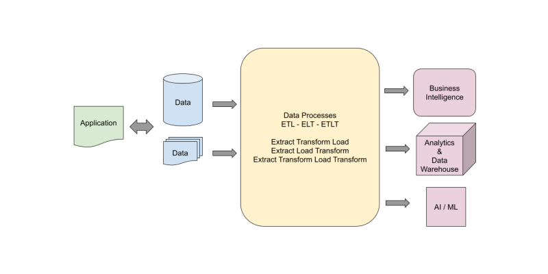
A data pipeline architecture is an integrated set of processes, tools, and infrastructure designed to automate the flow of data from its various sources to end destinations. It encompasses the end-to-end journey of data through collection, transformation, processing, and delivery stages.

The architecture defines how data is:

• Collected from diverse sources (databases, APIs, files, streaming platforms, IoT sensors)
• Processed and transformed to fit analytical needs
• Moved between systems efficiently and reliably
• Delivered to storage systems or consumption layers for analysis

Core Components

Every data pipeline architecture consists of several fundamental components:

1. Data Sources

The origins from which data is extracted, including:

• Relational databases (MySQL, PostgreSQL, Oracle)
• NoSQL databases (MongoDB, Cassandra)
• Cloud storage (Amazon S3, Azure Blob Storage, Google Cloud Storage)
• APIs and web services
• Flat files (CSV, JSON, XML)
• Streaming platforms (Apache Kafka, Amazon Kinesis)
• IoT devices and sensors
• SaaS applications

2. Ingestion Layer

The mechanism for extracting data from sources, supporting:

• Batch ingestion: Data collected at predefined intervals (hourly, daily, weekly)
• Real-time streaming ingestion: Continuous data flow as events occur
• Change Data Capture (CDC): Tracking and capturing changes in source systems
• API polling: Regular requests to external services

3. Transformation Engine

The processing layer where data is cleaned, enriched, and restructured:

• Data cleansing (removing duplicates, handling missing values)
• Data normalization and standardization
• Data enrichment (adding calculated fields, joining datasets)
• Aggregation and summarization
• Business logic application
• Format conversion

4. Data Storage

The destination systems where processed data resides:

• Data Warehouses: Structured storage optimized for analytics (Snowflake, Google BigQuery, Amazon Redshift, Azure Synapse)
• Data Lakes: Raw data storage in native format (Hadoop HDFS, Amazon S3, Azure Data Lake)
• Data Lakehouses: Hybrid architecture combining warehouse and lake capabilities (Databricks Delta Lake)
• Operational databases: For transactional workloads

5. Orchestration Layer

The coordination mechanism managing pipeline execution:

• Workflow scheduling and automation
• Dependency management
• Error handling and retry logic
• Resource allocation
• Popular tools: Apache Airflow, Prefect, Dagster, Azure Data Factory, AWS Step Functions

6. Monitoring and Observability

Systems tracking pipeline health and performance:

• Real-time metrics collection
• Logging and audit trails
• Alerting mechanisms
• Data quality validation
• Performance dashboards

---

Data Pipeline Lifecycle: Terminology Tables

Understanding the various terms used for pipeline stages is crucial for effective communication across teams and technologies.

Table 1: Pipeline Stage Terminology Equivalents

ETL Term	ELT Term	Streaming Term	General Pipeline Term	Description
Extract	Extract	Ingest	Collection	Retrieving data from source systems
Transform	Transform	Process	Processing	Applying business logic and data manipulation
Load	Load	Sink	Delivery	Moving data to destination systems
Staging Area	Landing Zone	Buffer	Intermediate Storage	Temporary data storage during processing
Data Warehouse	Data Warehouse	Data Store	Target System	Final destination for processed data
Source System	Source System	Producer	Origin	System generating or providing data
ETL Job	Pipeline Run	Stream Processing	Execution	Individual instance of pipeline processing
Schedule	Trigger	Event	Activation	Mechanism initiating pipeline execution
Validation	Data Quality Check	Validation	Quality Assurance	Verification of data correctness

Table 2: Hierarchical Differentiation of Pipeline Jargon

Level	Category	Terms	Scope	Technical Depth
Strategic	Architecture Pattern	ETL, ELT, EtLT, Lambda, Kappa, Medallion	Organization-wide	High-level design decisions
Tactical	Pipeline Type	Batch, Streaming, Micro-batch, Real-time, Near-real-time	Team/Project level	Implementation approach
Operational	Process Phase	Ingestion, Transformation, Loading, Validation, Monitoring	Daily operations	Execution steps
Technical	Component	Connector, Processor, Sink, Source, Orchestrator, Scheduler	Code/Configuration level	Specific tools and services
Data-Centric	Data State	Raw, Staged, Transformed, Curated, Consumption-ready	Data lifecycle	Data maturity stages
Quality-Focused	Validation Stage	Pre-ingestion, Post-ingestion, Pre-transformation, Post-transformation, Pre-load	Quality gates	Testing checkpoints
Infrastructure	Execution Mode	On-premises, Cloud-native, Hybrid, Multi-cloud, Serverless	Deployment model	Infrastructure choices

Table 3: Pattern-Specific Terminology

Architecture Pattern	Key Stages	Characteristic	Primary Use Case
ETL (Extract-Transform-Load)	Extract → Transform → Load	Transformation before loading	Small datasets, complex transformations, legacy systems
ELT (Extract-Load-Transform)	Extract → Load → Transform	Transformation after loading	Large datasets, cloud warehouses, flexible analysis
EtLT (Extract-light Transform-Load-Transform)	Extract → Light Transform → Load → Heavy Transform	Two-stage transformation	Hybrid scenarios, data lake to warehouse
Streaming (Stream-Process-Store)	Stream → Collect → Process → Store → Analyze	Continuous real-time processing	Real-time analytics, IoT, fraud detection
Lambda Architecture	Batch Layer + Speed Layer + Serving Layer	Parallel batch and stream processing	High-volume real-time with historical analysis
Kappa Architecture	Stream Processing Only	Pure streaming approach	Simplified real-time processing
Medallion Architecture	Bronze → Silver → Gold	Layered data refinement	Data lake organization, incremental quality improvement

---

Data Pipeline Architectures: Evolution and Types

Historical Evolution

Era 1: Traditional ETL (2000s-2010)

• Characteristics: On-premises infrastructure, limited storage, expensive compute
• Approach: Transform data before loading to optimize storage
• Limitation: Hardcoded pipelines, inflexible, time-consuming transformations
• Tools: Informatica, DataStage, SSIS

Era 2: Hadoop and Big Data (2011-2017)

• Innovation: Distributed processing, parallel computation
• Challenge: Still constrained by storage and compute limitations
• Evolution: Data modeling and query optimization remained critical
• Tools: Hadoop MapReduce, Hive, Pig

Era 3: Cloud Data Warehouses (2017-Present)

• Transformation: Unlimited scalable storage and compute
• Shift: ELT pattern becomes dominant
• Advantages: Load raw data first, transform as needed
• Tools: Snowflake, BigQuery, Redshift, Databricks

Era 4: Modern Data Stack (Present)

• Focus: Speed, agility, developer experience
• Features: Serverless, modular, API-driven
• Paradigm: Data-as-code, version control, CI/CD integration
• Tools: dbt, Fivetran, Airbyte, Modern orchestrators

ETL vs ELT: Detailed Comparison

ETL (Extract, Transform, Load)

Process Flow:

1. Extract: Data pulled from source systems
2. Transform: Data processed in staging area or transformation engine
   • Data cleansing and validation
   • Applying business rules
   • Normalization and standardization
   • Aggregations and calculations
3. Load: Transformed data loaded into target warehouse

Advantages:

• Reduced storage requirements in target system
• Data privacy and compliance (sensitive data can be filtered before loading)
• Optimized for legacy systems with limited processing power
• Predictable performance for specific use cases
• Better control over data quality before storage

Disadvantages:

• Longer time to insights (transformation adds latency)
• Less flexibility (must predict use cases upfront)
• Higher initial development complexity
• Difficult to adapt to changing requirements

Ideal Use Cases:

• Small to medium datasets
• Complex transformations required before loading
• Legacy data warehouses with storage constraints
• Regulatory requirements to exclude sensitive data
• On-premises infrastructure
• IoT edge computing scenarios

ELT (Extract, Load, Transform)

Process Flow:

1. Extract: Data pulled from source systems
2. Load: Raw data loaded directly into target system
   • All data types supported (structured, semi-structured, unstructured)
   • Minimal pre-processing
3. Transform: Data processed within the target system
   • Using in-database SQL transformations
   • Leveraging warehouse compute power
   • Transformation tools like dbt

Advantages:

• Faster time to value (immediate data availability)
• Greater flexibility (transform data as needed for any use case)
• Scalable with cloud-native architecture
• Raw data preservation for future analysis
• Simplified pipeline architecture

Disadvantages:

• Higher storage costs (storing all raw data)
• Requires powerful target system
• Data governance challenges
• Potential security concerns with raw sensitive data

Ideal Use Cases:

• Large datasets and big data scenarios
• Cloud-native data warehouses (Snowflake, BigQuery, Redshift)
• Need for flexible, ad-hoc analysis
• Machine learning and data science workflows
• Modern analytics requirements
• Organizations prioritizing speed over storage costs

Emerging Patterns

EtLT (Extract, Light Transform, Load, Heavy Transform)

A hybrid approach combining ETL and ELT benefits:

• Light transformation during extraction (basic cleansing)
• Load into data lake/staging area
• Heavy transformation in data warehouse
• Useful for complex multi-stage processing

Reverse ETL

Activating insights by pushing curated data back to operational systems:

• Extract from analytical stores (warehouses, lakehouses)
• Transform to operational format
• Load into business applications (CRM, marketing tools, support systems)
• Enables data-driven automation in operational workflows

Zero ETL

Minimizing traditional ETL overhead:

• Data cleaning and normalization before load
• Data remains in lake, queried in place
• Reduces data movement
• Challenges: Data governance, query performance

---

Building Secure Data Pipelines

Security must be embedded throughout the pipeline architecture, not added as an afterthought.

Security Principles

1. Defense in Depth

Implement multiple layers of security controls:

• Network security (VPCs, firewalls, security groups)
• Identity and access management
• Data encryption
• Application security
• Monitoring and auditing

2. Principle of Least Privilege

Grant minimum access necessary:

• Users receive only permissions required for their role
• Service accounts have limited, specific permissions
• Regular access reviews and revocation
• Time-bound access for temporary needs

3. Zero Trust Architecture

Assume no implicit trust:

• Verify every access request
• Authenticate and authorize continuously
• Segment network access
• Monitor all activity

Authentication and Authorization

Identity and Access Management (IAM)

Role-Based Access Control (RBAC):

• Define roles based on job functions (Data Engineer, Data Analyst, Data Scientist)
• Assign permissions to roles, not individuals
• Users inherit permissions from assigned roles
• Example role hierarchy:
  • Reader: Read-only access to processed data
  • Analyst: Read access to all data, write to analytical schemas
  • Engineer: Full pipeline development and deployment access
  • Admin: Full system administration capabilities

Attribute-Based Access Control (ABAC):

• Dynamic access based on attributes (department, project, data classification)
• More granular than RBAC
• Flexible for complex organizations

Multi-Factor Authentication (MFA)

Essential additional security layer:

• Knowledge factor: Something you know (password)
• Possession factor: Something you have (phone, hardware token)
• Inherence factor: Something you are (biometric)

Implementation examples:

• Time-based One-Time Passwords (TOTP)
• Hardware security keys (YubiKey)
• Biometric verification
• Push notifications to trusted devices

OAuth 2.0 and Single Sign-On (SSO)

For third-party integrations:

• Avoid storing credentials for external services
• Use access tokens with limited scope
• Implement token refresh and expiration
• Support for modern authentication flows

Managed Identities

For cloud services:

• No credential storage or management required
• Automatic credential rotation
• Azure Managed Identity, AWS IAM roles for service accounts, GCP Service Accounts

Data Encryption

Encryption at Rest

Protecting stored data:

Methods:

• Full Disk Encryption: Entire storage volume encrypted
• Database-level Encryption: Transparent Data Encryption (TDE)
• Column-level Encryption: Specific sensitive columns encrypted
• File-level Encryption: Individual files encrypted

Standards:

• AES-256 (Advanced Encryption Standard with 256-bit keys)
• Widely supported, government-approved
• Hardware-accelerated encryption available

Key Management:

• Use dedicated Key Management Services (KMS)
  • AWS KMS
  • Azure Key Vault
  • Google Cloud KMS
  • HashiCorp Vault
• Implement key rotation policies
• Separate key storage from encrypted data
• Support for customer-managed keys (CMK) and bring-your-own-key (BYOK)

Encryption in Transit

Protecting data during transmission:

Protocols:

• TLS 1.3 (Transport Layer Security): Latest standard for encrypted communication
• TLS 1.2: Minimum acceptable version, still widely supported
• Mutual TLS (mTLS): Both client and server authenticate each other

Implementation:

• Enforce HTTPS for all API communications
• Use secure protocols for database connections (SSL/TLS)
• VPN or private network connections for internal systems
• Certificate management and rotation

Data Masking and Tokenization

Additional protection for sensitive data:

Data Masking:

• Replace sensitive data with realistic but fake values
• Dynamic masking: Masked in real-time based on user permissions
• Static masking: Permanently masked in non-production environments

Tokenization:

• Replace sensitive data with non-sensitive tokens
• Original data stored securely in token vault
• Tokens useless if stolen without vault access

Network Security

Virtual Private Cloud (VPC)

Isolated network environment:

• Private subnets for sensitive resources
• Public subnets for internet-facing components
• Network Access Control Lists (NACLs)
• Security groups for resource-level firewalling

Private Endpoints and Service Endpoints

Avoid public internet exposure:

• Direct private connectivity to cloud services
• Bypass public internet entirely
• Reduce attack surface

Network Segmentation

Isolate pipeline components:

• Separate ingestion, processing, and storage networks
• Micro-segmentation for zero-trust implementation
• Network monitoring and intrusion detection

Secure Development Practices

Secrets Management

Never hardcode credentials:

Best Practices:

• Store secrets in dedicated secret managers (AWS Secrets Manager, HashiCorp Vault)
• Inject secrets at runtime via environment variables
• Implement secret rotation
• Audit secret access

Example (Conceptual):

# Bad - Hardcoded credentials
db_connection = "postgresql://user:password@host:5432/db"

# Good - Retrieved from secret manager
import os
db_host = os.environ['DB_HOST']
db_user = os.environ['DB_USER']
db_password = get_secret('database/password')

Code Security

• Input validation and sanitization to prevent injection attacks
• Parameterized queries to prevent SQL injection
• Regular dependency updates and vulnerability scanning
• Code review and security testing in CI/CD pipeline

Secure APIs

• Rate limiting to prevent abuse
• API authentication (API keys, OAuth tokens)
• Request validation
• API versioning and deprecation management

---

Monitoring and Observability

Effective monitoring ensures pipeline reliability, performance, and data quality.

Monitoring vs Observability

Monitoring:

• Tracking predefined metrics and thresholds
• Answering “Is something wrong?”
• Dashboard-based approach
• Focused on known issues

Observability:

• Understanding system internal state from external outputs
• Answering “Why is it wrong?”
• Exploratory analysis
• Discovering unknown issues
• Encompasses logs, metrics, and traces

Key Monitoring Metrics

Pipeline Health Metrics

1. Throughput:
   • Volume of data processed per unit time
   • Records per second/minute/hour
   • Gigabytes processed per day
   • Identifies bottlenecks and capacity issues
2. Latency:
   • Time to process individual records or batches
   • End-to-end pipeline execution time
   • Time between data generation and availability
   • Critical for SLA compliance
3. Error Rate:
   • Percentage of failed operations
   • Failed records vs total records
   • Error types and patterns
   • Alerts when thresholds exceeded
4. Data Freshness:
   • Time since last successful update
   • Age of most recent data
   • Critical for real-time analytics
   • Staleness indicators
5. Resource Utilization:
   • CPU usage
   • Memory consumption
   • Storage capacity
   • Network bandwidth
   • Cost tracking

Data Quality Metrics

1. Completeness:
   • Missing or null values
   • Record counts matching expectations
   • Required fields populated
2. Accuracy:
   • Data matching expected patterns
   • Validation rules compliance
   • Reference data conformity
3. Consistency:
   • Cross-system data matching
   • Referential integrity
   • No contradictions
4. Uniqueness:
   • Duplicate records
   • Primary key violations
   • Deduplication effectiveness
5. Validity:
   • Data type correctness
   • Format compliance
   • Range checks
6. Timeliness:
   • Data availability within expected windows
   • Update frequency meeting requirements

Monitoring Components

Logging

Structured Logging: Capture detailed information in parseable format:

• JSON or key-value format
• Include context (timestamp, pipeline ID, stage, user)
• Log levels (DEBUG, INFO, WARNING, ERROR, CRITICAL)
• Correlation IDs for tracing requests

Log Aggregation: Centralize logs from distributed systems:

• Tools: Elasticsearch, Splunk, Datadog, CloudWatch
• Search and filter capabilities
• Long-term retention for compliance

Example (Conceptual):

import logging
import json

logger = logging.getLogger('data-pipeline')

def process_batch(batch_id, data):
    logger.info(json.dumps({
        'event': 'batch_processing_started',
        'batch_id': batch_id,
        'record_count': len(data),
        'timestamp': datetime.now().isoformat()
    }))
    
    try:
        result = transform_data(data)
        logger.info(json.dumps({
            'event': 'batch_processing_completed',
            'batch_id': batch_id,
            'success_count': result.success_count,
            'timestamp': datetime.now().isoformat()
        }))
    except Exception as e:
        logger.error(json.dumps({
            'event': 'batch_processing_failed',
            'batch_id': batch_id,
            'error': str(e),
            'timestamp': datetime.now().isoformat()
        }))
        raise

Alerting

Alert Configuration:

• Define meaningful thresholds
• Avoid alert fatigue with appropriate sensitivity
• Prioritize alerts by severity
• Include actionable context

Alert Channels:

• Email for non-urgent issues
• SMS/phone for critical failures
• Slack/Teams for team notifications
• PagerDuty for on-call escalation
• Automated remediation for known issues

Alert Types:

• Threshold-based (metric exceeds limit)
• Anomaly detection (ML-based pattern recognition)
• Trend-based (gradual degradation)
• Composite (multiple conditions)

Dashboards

Operational Dashboards: Real-time pipeline status:

• Current pipeline runs
• Active errors and warnings
• Resource utilization
• Data freshness indicators

Analytical Dashboards: Historical trends and patterns:

• Processing time trends
• Error rate evolution
• Data volume growth
• Cost analysis

Tools:

• Grafana: Open-source, flexible visualization
• Datadog: Comprehensive observability platform
• Prometheus + Grafana: Metrics collection and visualization
• CloudWatch Dashboards: AWS native
• Azure Monitor: Azure native

Data Lineage and Impact Analysis

Data Lineage: Tracking data flow through systems:

• Source to destination tracing
• Transformation history
• Dependency mapping
• Compliance documentation

Impact Analysis: Understanding downstream effects:

• Identifying affected systems when issues occur
• Planning change impacts
• Root cause analysis
• Priority determination

Tools:

• Alation
• Collibra
• Apache Atlas
• AWS Glue Data Catalog
• dbt documentation

---

Data Quality and Testing

Ensuring data quality throughout the pipeline lifecycle.

Testing Strategies

1. Shift-Left Testing

Catch issues early in the pipeline:

Pre-Ingestion Validation:

• Schema validation at source
• Data contracts between producers and consumers
• API response validation

Ingestion-Time Validation:

• Format verification
• Required field checks
• Basic data type validation

Advantages:

• Prevent bad data from entering pipeline
• Reduce downstream troubleshooting
• Lower remediation costs

2. Multi-Layer Validation

Source Table Validation:

• Circuit-breaker checks (halt pipeline if critical issues detected)
  • Row count within expected range
  • Join key completeness
  • Critical business metrics validation
• Warning checks (log but don’t halt)
  • Non-critical quality issues
  • Investigation during business hours

Transformation Validation:

• Pre-transformation checks (validate inputs)
• Post-transformation checks (validate outputs)
• Transformation logic correctness

Target Table Validation:

• Final data quality verification
• Business rule compliance
• Completeness and consistency checks

3. Testing Types

Unit Tests: Test individual transformation functions:

def test_data_transformation():
    input_data = [
        {'id': 1, 'value': 10},
        {'id': 2, 'value': 20}
    ]
    expected_output = [
        {'id': 1, 'value': 10, 'doubled': 20},
        {'id': 2, 'value': 20, 'doubled': 40}
    ]
    
    actual_output = apply_doubling_transformation(input_data)
    
    assert actual_output == expected_output

Integration Tests: Test pipeline components working together:

• End-to-end data flow verification
• System interaction validation
• Dependency testing

Contract Tests: Validate interfaces between systems:

• API contract compliance
• Schema agreement between producer/consumer
• Data format expectations

Data Quality Tests: Validate data characteristics:

• Null value checks
• Uniqueness constraints
• Range validations
• Business rule compliance
• Statistical distribution checks

Data Quality Frameworks

Great Expectations

Declarative data validation framework:

Expectations: Define rules about data:

# Example expectations (conceptual)
df.expect_column_to_exist("customer_id")
df.expect_column_values_to_not_be_null("customer_id")
df.expect_column_values_to_be_unique("customer_id")
df.expect_column_values_to_be_between("age", min_value=0, max_value=120)
df.expect_column_values_to_be_in_set("status", ["active", "inactive", "pending"])

Validation Results:

• Pass/fail for each expectation
• Summary statistics
• Data profiling
• Integration with orchestration tools

dbt Tests

SQL-based testing in transformation layer:

Built-in Tests:

• unique: Column values must be unique
• not_null: Column must not contain null values
• accepted_values: Column values must be in specified set
• relationships: Foreign key validation

Custom Tests: SQL queries returning failing records:

-- Custom test for valid email format
SELECT *
FROM 
WHERE email NOT LIKE '%@%.%'

Data Quality Monitoring

Automated Data Profiling

Understand data characteristics:

• Statistical summaries (min, max, mean, median, standard deviation)
• Distribution analysis
• Cardinality (unique value counts)
• Pattern recognition

Anomaly Detection

Identify unexpected data behavior:

• Statistical methods (Z-score, IQR)
• Machine learning models
• Time-series analysis
• Baseline comparison

Data Quality Dashboards

Visualize quality metrics over time:

• Completeness trends
• Error rates
• Schema change tracking
• Data drift detection

---

Best Practices for Robust Data Pipelines

1. Design for Scalability

Horizontal Scaling:

• Add more nodes/workers to handle increased load
• Distribute processing across multiple machines
• Use parallel processing where possible

Data Partitioning:

• Split large datasets into smaller, manageable chunks
• Partition by date, geography, or other logical dimensions
• Enable parallel processing of partitions

Modular Architecture:

• Design independent, reusable components
• Scale specific components as needed
• Easier maintenance and updates

Cloud Resource Optimization:

• Use auto-scaling for dynamic workloads
• Leverage spot instances for cost savings
• Right-size compute resources based on actual needs

2. Implement Idempotency

Definition: Pipeline execution produces the same result regardless of how many times it’s run with the same input.

Techniques:

• Unique transaction IDs for deduplication
• Upsert (update or insert) operations instead of append-only
• Timestamp-based processing (process only new data since last run)
• Atomic operations and transactions

Benefits:

• Safe retries after failures
• Consistent results
• Simplified error recovery

3. Handle Errors Gracefully

Error Detection:

• Comprehensive exception handling
• Validation at each stage
• Timeout configurations

Error Categorization:

• Transient errors: Temporary issues (network glitches) - retry automatically
• Data errors: Bad data quality - log, quarantine, and alert
• System errors: Infrastructure problems - escalate immediately
• Logic errors: Code bugs - halt pipeline, alert developers

Retry Mechanisms:

• Exponential backoff (increasing delay between retries)
• Maximum retry limits
• Circuit breakers (stop retrying after threshold)

Dead Letter Queues:

• Store failed messages for later analysis
• Prevent blocking of pipeline
• Enable manual intervention

Self-Healing:

• Automated remediation for common issues
• Automatic resource reallocation
• Fallback mechanisms

4. Version Control and CI/CD

Version Control:

• Store all pipeline code in Git
• Branch strategy (main, development, feature branches)
• Code review process
• Commit message standards

Continuous Integration:

• Automated testing on every commit
• Linting and code quality checks
• Security scanning
• Build validation

Continuous Deployment:

• Automated deployment to environments (dev, staging, production)
• Rollback capabilities
• Blue-green or canary deployments
• Infrastructure as Code (Terraform, CloudFormation)

Benefits:

• Reproducible deployments
• Faster development cycles
• Reduced human error
• Audit trail of changes

5. Documentation and Data Governance

Pipeline Documentation:

• Architecture diagrams
• Data flow documentation
• Transformation logic explanation
• Dependency mapping
• Runbooks for common issues

Data Catalog:

• Metadata management
• Data dictionary
• Business glossary
• Data lineage documentation
• Data ownership and stewardship

Data Contracts:

• Schema agreements between teams
• SLA definitions
• Data quality expectations
• Change management procedures

6. Cost Optimization

Storage Optimization:

• Data lifecycle policies (move old data to cheaper storage)
• Compression and efficient file formats (Parquet, ORC)
• Deduplication and archival
• Data retention policies

Compute Optimization:

• Right-sizing resources
• Scheduled scaling (scale down during off-hours)
• Caching frequently accessed data
• Query optimization

Cost Monitoring:

• Budget alerts
• Cost allocation tags
• Regular cost reviews
• ROI analysis

7. Compliance and Privacy

Regulatory Compliance:

• GDPR (General Data Protection Regulation)
• HIPAA (Health Insurance Portability and Accountability Act)
• CCPA (California Consumer Privacy Act)
• SOC 2 (Service Organization Control 2)
• Industry-specific regulations

Data Classification:

• Public data
• Internal data
• Confidential data
• Restricted data (PII, PHI, PCI)

Privacy by Design:

• Data minimization (collect only what’s needed)
• Purpose limitation (use data only for stated purpose)
• Right to erasure implementation
• Consent management
• Privacy impact assessments

Audit Trails:

• Comprehensive logging of data access
• Change tracking
• Compliance reporting
• Regular audits

---

Modern Data Pipeline Tools and Technologies

Orchestration Tools

Tool	Type	Strengths	Best For
Apache Airflow	Open-source	Mature, extensive community, Python-based DAGs	Complex workflows, large teams
Prefect	Open-source/Cloud	Modern UI, dynamic workflows, failure recovery	Developer experience, observability
Dagster	Open-source	Software-defined assets, testing framework	Data apps, version control
Azure Data Factory	Cloud-native	Azure integration, visual interface, 90+ connectors	Azure ecosystem
AWS Step Functions	Cloud-native	Serverless, AWS service integration	AWS workflows, event-driven
Google Cloud Composer	Managed Airflow	Fully managed, GCP integration	Google Cloud users

Data Integration Tools

Tool	Type	Approach	Strengths
Fivetran	Commercial	Automated ELT	Pre-built connectors, minimal maintenance
Airbyte	Open-source	ELT	Extensive connectors, customizable, self-hosted
Stitch	Commercial	ELT	Simple setup, quick deployment
Apache NiFi	Open-source	Data flow	Visual interface, real-time processing
Talend	Commercial	ETL/ELT	Enterprise features, data quality

Transformation Tools

Tool	Type	Language	Strengths
dbt (data build tool)	Open-source	SQL	Transformation as code, testing, documentation
Apache Spark	Open-source	Scala/Python	Distributed processing, large-scale data
Databricks	Commercial	Spark-based	Unified analytics, notebooks, collaboration
AWS Glue	Cloud-native	Python/Scala	Serverless, AWS integration, Data Catalog

Streaming Platforms

Tool	Type	Strengths	Use Cases
Apache Kafka	Open-source	High throughput, durability, ecosystem	Event streaming, log aggregation
Amazon Kinesis	Cloud-native	AWS integration, managed, auto-scaling	Real-time analytics, AWS ecosystem
Apache Flink	Open-source	Complex event processing, exactly-once semantics	Stateful stream processing
Apache Pulsar	Open-source	Multi-tenancy, geo-replication	Cloud-native streaming

Storage Solutions

Solution	Type	Architecture	Best For
Snowflake	Cloud Warehouse	Decoupled compute/storage	Analytics, ease of use, scalability
Google BigQuery	Cloud Warehouse	Serverless	Ad-hoc queries, Google Cloud, cost efficiency
Amazon Redshift	Cloud Warehouse	Columnar storage	AWS ecosystem, large datasets
Databricks Lakehouse	Lakehouse	Delta Lake	Unified analytics, ML/AI workloads
Azure Synapse	Cloud Warehouse	Integrated analytics	Azure ecosystem, hybrid workloads
Amazon S3	Object Storage	Data Lake	Raw data storage, cost-effective

---

Implementation Patterns and Examples

Pattern 1: Batch ETL Pipeline

Scenario: Daily customer data synchronization from operational database to data warehouse

Architecture:

1. Extract customer records modified in last 24 hours
2. Transform: Apply business rules, enrich with reference data
3. Load into data warehouse dimension tables
4. Update slowly changing dimensions (SCD Type 2)

Implementation Approach (Conceptual):

from airflow import DAG
from airflow.operators.python import PythonOperator
from datetime import datetime, timedelta
import pandas as pd

# DAG Definition
default_args = {
    'owner': 'data-engineering',
    'depends_on_past': False,
    'start_date': datetime(2024, 1, 1),
    'email_on_failure': True,
    'email_on_retry': False,
    'retries': 3,
    'retry_delay': timedelta(minutes=5),
}

dag = DAG(
    'customer_etl_daily',
    default_args=default_args,
    description='Daily customer ETL pipeline',
    schedule_interval='0 2 * * *',  # Run at 2 AM daily
    catchup=False
)

def extract_customers(**context):
    """Extract customers modified in last 24 hours"""
    execution_date = context['execution_date']
    
    # Query source database
    query = f"""
        SELECT customer_id, name, email, phone, address, 
               city, state, country, created_at, updated_at
        FROM customers
        WHERE updated_at >= '{execution_date - timedelta(days=1)}'
    """
    
    # Execute query and save to staging
    df = execute_database_query(query)
    df.to_parquet(f'/staging/customers_{execution_date}.parquet')
    
    return f'/staging/customers_{execution_date}.parquet'

def transform_customers(**context):
    """Transform and enrich customer data"""
    ti = context['task_instance']
    staging_file = ti.xcom_pull(task_ids='extract')
    
    df = pd.read_parquet(staging_file)
    
    # Data cleansing
    df['email'] = df['email'].str.lower().str.strip()
    df['phone'] = df['phone'].str.replace(r'\D', '', regex=True)
    
    # Data enrichment
    # Add customer segment based on business rules
    df['segment'] = df.apply(calculate_customer_segment, axis=1)
    
    # Add data quality flags
    df['email_valid'] = df['email'].str.contains('@')
    df['phone_valid'] = df['phone'].str.len() == 10
    
    # Add metadata
    df['etl_timestamp'] = datetime.now()
    df['etl_batch_id'] = context['run_id']
    
    transformed_file = staging_file.replace('staging', 'transformed')
    df.to_parquet(transformed_file)
    
    return transformed_file

def validate_data(**context):
    """Validate transformed data quality"""
    ti = context['task_instance']
    transformed_file = ti.xcom_pull(task_ids='transform')
    
    df = pd.read_parquet(transformed_file)
    
    # Quality checks
    checks = {
        'null_customer_id': df['customer_id'].isnull().sum(),
        'duplicate_customer_id': df['customer_id'].duplicated().sum(),
        'invalid_email': (~df['email_valid']).sum(),
        'total_records': len(df)
    }
    
    # Log quality metrics
    log_quality_metrics(checks)
    
    # Circuit breaker: Halt if critical issues found
    if checks['null_customer_id'] > 0:
        raise ValueError("Critical: Null customer IDs found")
    
    if checks['duplicate_customer_id'] > 0:
        raise ValueError("Critical: Duplicate customer IDs found")
    
    # Warning for non-critical issues
    if checks['invalid_email'] > checks['total_records'] * 0.1:
        log_warning(f"High invalid email rate: {checks['invalid_email']}")
    
    return True

def load_to_warehouse(**context):
    """Load data to data warehouse with SCD Type 2"""
    ti = context['task_instance']
    transformed_file = ti.xcom_pull(task_ids='transform')
    
    df = pd.read_parquet(transformed_file)
    
    # Implement SCD Type 2 logic
    for _, row in df.iterrows():
        # Check if customer exists in warehouse
        existing = query_warehouse(
            f"SELECT * FROM dim_customer WHERE customer_id = {row['customer_id']} AND is_current = 1"
        )
        
        if existing.empty:
            # New customer - insert
            insert_to_warehouse('dim_customer', row, is_current=1)
        else:
            # Check if data changed
            if has_changes(existing, row):
                # Expire old record
                update_warehouse(
                    'dim_customer',
                    {'is_current': 0, 'end_date': datetime.now()},
                    f"customer_id = {row['customer_id']} AND is_current = 1"
                )
                # Insert new record
                insert_to_warehouse('dim_customer', row, is_current=1)

# Define task dependencies
extract_task = PythonOperator(
    task_id='extract',
    python_callable=extract_customers,
    dag=dag
)

transform_task = PythonOperator(
    task_id='transform',
    python_callable=transform_customers,
    dag=dag
)

validate_task = PythonOperator(
    task_id='validate',
    python_callable=validate_data,
    dag=dag
)

load_task = PythonOperator(
    task_id='load',
    python_callable=load_to_warehouse,
    dag=dag
)

# Set task execution order
extract_task >> transform_task >> validate_task >> load_task

Key Features:

• Incremental extraction (only changed records)
• Multi-stage transformation
• Data quality validation with circuit breakers
• Slowly Changing Dimension (SCD Type 2) implementation
• Retry logic and error handling
• Metadata tracking

Pattern 2: Real-Time Streaming Pipeline

Scenario: Processing clickstream events for real-time analytics and personalization

Architecture:

1. Web/mobile apps send events to Kafka
2. Stream processor (Flink/Spark Streaming) processes events
3. Enrich with user profile data
4. Write to real-time database (Redis) and data warehouse

Implementation Approach (Conceptual):

from pyspark.sql import SparkSession
from pyspark.sql.functions import from_json, col, window, count, avg
from pyspark.sql.types import StructType, StringType, TimestampType, IntegerType

# Initialize Spark with Kafka support
spark = SparkSession.builder \
    .appName("ClickstreamProcessor") \
    .config("spark.jars.packages", "org.apache.spark:spark-sql-kafka-0-10_2.12:3.5.0") \
    .getOrCreate()

# Define event schema
event_schema = StructType() \
    .add("event_id", StringType()) \
    .add("user_id", StringType()) \
    .add("session_id", StringType()) \
    .add("event_type", StringType()) \
    .add("page_url", StringType()) \
    .add("timestamp", TimestampType()) \
    .add("device_type", StringType()) \
    .add("properties", StringType())

# Read from Kafka
raw_events = spark \
    .readStream \
    .format("kafka") \
    .option("kafka.bootstrap.servers", "kafka-broker:9092") \
    .option("subscribe", "clickstream-events") \
    .option("startingOffsets", "latest") \
    .load()

# Parse JSON events
parsed_events = raw_events \
    .select(from_json(col("value").cast("string"), event_schema).alias("data")) \
    .select("data.*")

# Data quality filtering
valid_events = parsed_events \
    .filter(col("event_id").isNotNull()) \
    .filter(col("user_id").isNotNull()) \
    .filter(col("timestamp").isNotNull())

# Enrich with user data (join with slowly changing user profile)
enriched_events = valid_events \
    .join(
        spark.read.table("user_profiles"),
        on="user_id",
        how="left"
    ) \
    .select(
        "event_id", "user_id", "session_id", "event_type",
        "page_url", "timestamp", "device_type",
        "user_segment", "user_country", "user_subscription_tier"
    )

# Real-time aggregations (5-minute tumbling windows)
event_metrics = enriched_events \
    .withWatermark("timestamp", "10 minutes") \
    .groupBy(
        window("timestamp", "5 minutes"),
        "event_type",
        "user_segment"
    ) \
    .agg(
        count("*").alias("event_count"),
        count("user_id").alias("unique_users")
    )

# Write enriched events to data warehouse (append mode)
warehouse_writer = enriched_events \
    .writeStream \
    .format("delta") \
    .outputMode("append") \
    .option("checkpointLocation", "/checkpoints/clickstream") \
    .option("path", "s3://data-lake/clickstream/events/") \
    .trigger(processingTime="30 seconds") \
    .start()

# Write real-time metrics to Redis for dashboards
def write_to_redis(batch_df, batch_id):
    """Write batch to Redis for real-time access"""
    for row in batch_df.collect():
        window_start = row['window']['start']
        key = f"metrics:{row['event_type']}:{row['user_segment']}:{window_start}"
        
        redis_client.setex(
            key,
            3600,  # Expire after 1 hour
            json.dumps({
                'event_count': row['event_count'],
                'unique_users': row['unique_users'],
                'window_start': str(window_start)
            })
        )

metrics_writer = event_metrics \
    .writeStream \
    .foreachBatch(write_to_redis) \
    .outputMode("update") \
    .trigger(processingTime="10 seconds") \
    .start()

# Wait for termination
spark.streams.awaitAnyTermination()

Key Features:

• Stream processing with Spark Structured Streaming
• Schema definition and validation
• Data enrichment with dimension tables
• Watermarking for handling late data
• Windowed aggregations
• Multi-sink output (warehouse + cache)
• Checkpointing for fault tolerance

Pattern 3: ELT with dbt

Scenario: Transforming raw sales data into analytics-ready models

Project Structure:

dbt_project/
├── models/
│   ├── staging/
│   │   ├── stg_orders.sql
│   │   └── stg_customers.sql
│   ├── intermediate/
│   │   └── int_order_items_enriched.sql
│   └── marts/
│       ├── fct_orders.sql
│       └── dim_customers.sql
├── tests/
│   └── assert_positive_order_total.sql
├── macros/
│   └── cents_to_dollars.sql
└── dbt_project.yml

Staging Model (stg_orders.sql):

-- Staging layer: Clean and standardize raw data



WITH source AS (
    SELECT * FROM 
),

cleaned AS (
    SELECT
        order_id,
        customer_id,
        order_date,
         AS order_total,
        order_status,
        UPPER(TRIM(shipping_country)) AS shipping_country,
        LOWER(TRIM(payment_method)) AS payment_method,
        created_at,
        updated_at,
        
        -- Data quality flags
        CASE
            WHEN order_total_cents <= 0 THEN FALSE
            ELSE TRUE
        END AS is_valid_amount,
        
        CASE
            WHEN order_status IN ('completed', 'pending', 'cancelled', 'refunded') THEN TRUE
            ELSE FALSE
        END AS is_valid_status
        
    FROM source
    WHERE order_date >= '2020-01-01'  -- Historical cutoff
)

SELECT * FROM cleaned

Intermediate Model (int_order_items_enriched.sql):

-- Intermediate layer: Business logic and enrichment



WITH orders AS (
    SELECT * FROM 
),

order_items AS (
    SELECT * FROM 
),

products AS (
    SELECT * FROM 
),

enriched AS (
    SELECT
        oi.order_item_id,
        oi.order_id,
        o.customer_id,
        o.order_date,
        o.order_status,
        
        oi.product_id,
        p.product_name,
        p.product_category,
        p.product_subcategory,
        
        oi.quantity,
        oi.unit_price,
        oi.quantity * oi.unit_price AS line_total,
        
        -- Business calculations
        CASE
            WHEN oi.quantity >= 10 THEN 'bulk'
            WHEN oi.quantity >= 5 THEN 'moderate'
            ELSE 'single'
        END AS quantity_tier,
        
        p.cost_price,
        (oi.unit_price - p.cost_price) * oi.quantity AS line_profit
        
    FROM order_items oi
    INNER JOIN orders o ON oi.order_id = o.order_id
    INNER JOIN products p ON oi.product_id = p.product_id
    WHERE o.is_valid_amount AND o.is_valid_status
)

SELECT * FROM enriched

Mart Model (fct_orders.sql):

-- Mart layer: Final analytical model



WITH order_items AS (
    SELECT * FROM 
),

order_aggregates AS (
    SELECT
        order_id,
        customer_id,
        order_date,
        order_status,
        
        -- Aggregated metrics
        COUNT(DISTINCT product_id) AS product_count,
        SUM(quantity) AS total_quantity,
        SUM(line_total) AS order_total,
        SUM(line_profit) AS order_profit,
        
        -- Product mix
        COUNT(DISTINCT product_category) AS category_count,
        LISTAGG(DISTINCT product_category, ', ') AS categories,
        
        -- Profitability metrics
        SUM(line_profit) / NULLIF(SUM(line_total), 0) AS profit_margin
        
    FROM order_items
    GROUP BY 1, 2, 3, 4
),

final AS (
    SELECT
        order_id,
        customer_id,
        order_date,
        order_status,
        product_count,
        total_quantity,
        order_total,
        order_profit,
        profit_margin,
        category_count,
        categories,
        
        -- Categorization
        CASE
            WHEN order_total >= 1000 THEN 'high_value'
            WHEN order_total >= 100 THEN 'medium_value'
            ELSE 'low_value'
        END AS order_value_tier,
        
        CURRENT_TIMESTAMP AS dbt_updated_at
        
    FROM order_aggregates
    
    
)

SELECT * FROM final

Custom Test (assert_positive_order_total.sql):

-- tests/assert_positive_order_total.sql
-- Custom data quality test

SELECT
    order_id,
    order_total
FROM 
WHERE order_total <= 0

Schema Definition (schema.yml):

version: 2

models:
  - name: fct_orders
    description: "Fact table containing order-level metrics and dimensions"
    columns:
      - name: order_id
        description: "Unique identifier for each order"
        tests:
          - unique
          - not_null
      
      - name: customer_id
        description: "Foreign key to dim_customers"
        tests:
          - not_null
          - relationships:
              to: ref('dim_customers')
              field: customer_id
      
      - name: order_date
        description: "Date when order was placed"
        tests:
          - not_null
      
      - name: order_total
        description: "Total order amount in dollars"
        tests:
          - not_null
          - dbt_utils.expression_is_true:
              expression: ">= 0"
      
      - name: order_status
        description: "Current status of the order"
        tests:
          - not_null
          - accepted_values:
              values: ['completed', 'pending', 'cancelled', 'refunded']

Key Features:

• Layered architecture (staging → intermediate → marts)
• Incremental materialization for efficiency
• Built-in and custom data quality tests
• Macros for reusable logic
• Documentation and data lineage
• Version control friendly (SQL files)

---

Advanced Topics

Change Data Capture (CDC)

What is CDC? Change Data Capture is a technique for tracking and capturing changes (inserts, updates, deletes) in source systems and propagating them to target systems efficiently.

Why CDC?

• Reduces load on source systems (no full table scans)
• Near real-time data synchronization
• Captures deletes (impossible with timestamp-based extraction)
• Lower network bandwidth usage
• Better scalability

CDC Approaches:

1. Log-Based CDC: Reads database transaction logs (most efficient):

• MySQL: Binary logs (binlog)
• PostgreSQL: Write-Ahead Logging (WAL)
• Oracle: Redo logs
• SQL Server: Transaction log

Advantages:

• No impact on source system performance
• Captures all changes including deletes
• No schema modifications required

Tools:

• Debezium (open-source)
• AWS DMS (Database Migration Service)
• Fivetran
• Qlik Replicate

2. Trigger-Based CDC: Database triggers capture changes to shadow tables:

-- Example trigger for CDC
CREATE TRIGGER customer_cdc_trigger
AFTER INSERT OR UPDATE OR DELETE ON customers
FOR EACH ROW
BEGIN
    IF INSERTING THEN
        INSERT INTO customers_cdc (operation, customer_id, data, timestamp)
        VALUES ('INSERT', :NEW.customer_id, :NEW, CURRENT_TIMESTAMP);
    ELSIF UPDATING THEN
        INSERT INTO customers_cdc (operation, customer_id, data, timestamp)
        VALUES ('UPDATE', :NEW.customer_id, :NEW, CURRENT_TIMESTAMP);
    ELSIF DELETING THEN
        INSERT INTO customers_cdc (operation, customer_id, data, timestamp)
        VALUES ('DELETE', :OLD.customer_id, :OLD, CURRENT_TIMESTAMP);
    END IF;
END;

Advantages:

• Works with any database supporting triggers
• Customizable logic

Disadvantages:

• Performance overhead on source system
• Schema modifications required
• Complex trigger management

3. Timestamp/Version-Based CDC: Using last_modified timestamp or version columns:

-- Incremental extraction
SELECT *
FROM customers
WHERE updated_at > :last_extraction_time

Advantages:

• Simple to implement
• No special tools required

Disadvantages:

• Cannot capture deletes
• Requires schema modifications
• Can miss rapid updates within same timestamp

Data Lakehouse Architecture

What is a Lakehouse? A unified architecture combining the best features of data lakes and data warehouses:

• From Data Lakes: Low-cost storage, support for all data types, scalability
• From Data Warehouses: ACID transactions, schema enforcement, query performance

Key Technologies:

Delta Lake (Databricks):

• ACID transactions on data lakes
• Time travel (query historical data)
• Schema evolution and enforcement
• Unified batch and streaming
• Data versioning

Apache Iceberg:

• Open table format
• Hidden partitioning
• Time travel and rollback
• Schema evolution
• Multi-engine support (Spark, Flink, Trino)

Apache Hudi:

• Incremental processing
• Update/delete support on data lakes
• Timeline for data versioning
• Optimized for streaming

Medallion Architecture: Organizing lakehouse in layers:

Bronze Layer (Raw):

• Raw ingested data in native format
• No transformations
• Complete history preserved
• Append-only

Silver Layer (Cleansed and Conformed):

• Cleaned and validated data
• Standardized formats
• Deduplication
• Business key integration
• May contain PII

Gold Layer (Business-Level Aggregates):

• Highly refined, aggregate data
• Business-level metrics and KPIs
• Optimized for consumption
• Powers dashboards and reports

Example Structure:

bronze/
  ├── source_system_1/
  │   ├── table_a/
  │   └── table_b/
  └── source_system_2/

silver/
  ├── customers/
  ├── orders/
  └── products/

gold/
  ├── sales_metrics/
  ├── customer_360/
  └── inventory_summary/

Data Mesh Architecture

Concept: Decentralized data ownership where domain teams own and serve their data products.

Four Principles:

1. Domain-Oriented Ownership:

• Data owned by domain teams, not central IT
• Domain expertise embedded in data products
• Autonomous teams

2. Data as a Product:

• Treat data with product thinking
• SLAs and quality guarantees
• Self-service discovery
• Documentation and metadata

3. Self-Serve Data Infrastructure:

• Platform team provides infrastructure
• Domain teams use infrastructure independently
• Automated tooling

4. Federated Computational Governance:

• Global standards and policies
• Automated enforcement
• Decentralized implementation

Implementation Considerations:

• Requires organizational maturity
• Clear domain boundaries
• Strong platform capabilities
• Cultural shift needed

---

Performance Optimization

Query Optimization

1. Partitioning: Divide data into smaller, manageable segments:

-- Partitioned table by date
CREATE TABLE orders (
    order_id INT,
    customer_id INT,
    order_date DATE,
    order_total DECIMAL
)
PARTITION BY RANGE (order_date) (
    PARTITION p_2024_01 VALUES LESS THAN ('2024-02-01'),
    PARTITION p_2024_02 VALUES LESS THAN ('2024-03-01'),
    PARTITION p_2024_03 VALUES LESS THAN ('2024-04-01')
);

-- Query only scans relevant partitions
SELECT * FROM orders
WHERE order_date BETWEEN '2024-02-01' AND '2024-02-28';

Benefits:

• Partition pruning (scan only relevant partitions)
• Parallel processing
• Easier maintenance
• Improved query performance

2. Indexing: Create indexes on frequently queried columns:

-- B-tree index for equality and range queries
CREATE INDEX idx_customer_id ON orders(customer_id);

-- Composite index for multi-column queries
CREATE INDEX idx_customer_date ON orders(customer_id, order_date);

-- Covering index includes all query columns
CREATE INDEX idx_covering ON orders(customer_id, order_date, order_total);

3. Materialized Views: Pre-compute expensive aggregations:

CREATE MATERIALIZED VIEW daily_sales_summary AS
SELECT
    order_date,
    COUNT(*) AS order_count,
    SUM(order_total) AS total_sales,
    AVG(order_total) AS avg_order_value
FROM orders
GROUP BY order_date;

-- Refresh periodically
REFRESH MATERIALIZED VIEW daily_sales_summary;

4. Query Pushdown: Push filtering and aggregation to source:

# Bad: Read all data then filter
df = spark.read.jdbc(url, "orders")
filtered = df.filter(col("order_date") == "2024-01-01")

# Good: Filter at source
df = spark.read.jdbc(
    url, 
    "orders",
    predicates=["order_date = '2024-01-01'"]
)

Storage Optimization

1. Columnar Formats: Store data by column instead of row:

Parquet:

• Excellent compression
• Column-level operations efficient
• Supports complex nested data
• Industry standard

ORC (Optimized Row Columnar):

• Better compression than Parquet
• Lightweight indexes
• Optimized for Hive

Comparison:

# CSV: 1.2 GB
# Parquet with compression: 150 MB (8x reduction)
# Query time: 10x faster with Parquet

df.write.parquet("data.parquet", compression="snappy")

2. Compression: Reduce storage footprint:

Algorithm	Compression Ratio	Speed	Use Case
Snappy	Low	Very Fast	Default for Parquet
GZIP	Medium	Medium	Balanced
ZSTD	High	Fast	Modern choice
LZ4	Low	Fastest	Real-time systems

3. Data Pruning: Eliminate unnecessary data:

• Drop unused columns early
• Filter rows at source
• Avoid SELECT *
• Use column projection

Parallel Processing

1. Data Parallelism: Process multiple data partitions simultaneously:

# Spark automatically parallelizes
df = spark.read.parquet("large_dataset")
result = df.groupBy("category").agg(sum("amount"))
# Executes across multiple executors in parallel

2. Task Parallelism: Execute independent tasks concurrently:

# Airflow parallel execution
with DAG('parallel_processing') as dag:
    start = DummyOperator(task_id='start')
    end = DummyOperator(task_id='end')
    
    # These run in parallel
    task1 = PythonOperator(task_id='process_source_1', ...)
    task2 = PythonOperator(task_id='process_source_2', ...)
    task3 = PythonOperator(task_id='process_source_3', ...)
    
    start >> [task1, task2, task3] >> end

3. Resource Tuning: Optimize cluster resources:

# Spark configuration
spark = SparkSession.builder \
    .config("spark.executor.memory", "4g") \
    .config("spark.executor.cores", "4") \
    .config("spark.sql.shuffle.partitions", "200") \
    .config("spark.default.parallelism", "200") \
    .getOrCreate()

---

Disaster Recovery and Business Continuity

Backup Strategies

1. Regular Backups:

• Full backups: Complete copy of all data
• Incremental backups: Only changed data since last backup
• Differential backups: Changes since last full backup

Frequency:

• Critical data: Hourly or continuous
• Important data: Daily
• Archival data: Weekly or monthly

2. Backup Storage:

• 3-2-1 Rule: 3 copies, 2 different media types, 1 offsite
• Geographic redundancy
• Immutable backups (protect against ransomware)

3. Retention Policies:

Daily backups: Keep for 7 days
Weekly backups: Keep for 4 weeks
Monthly backups: Keep for 12 months
Yearly backups: Keep for 7 years (compliance)

Recovery Strategies

Recovery Time Objective (RTO): Maximum acceptable downtime:

• Tier 1 (Critical): < 1 hour
• Tier 2 (Important): < 4 hours
• Tier 3 (Normal): < 24 hours

Recovery Point Objective (RPO): Maximum acceptable data loss:

• Tier 1: Near-zero (continuous replication)
• Tier 2: < 1 hour
• Tier 3: < 24 hours

High Availability Architectures:

Active-Passive:

• Primary system handles all traffic
• Standby system ready for failover
• Regular health checks
• Automated or manual failover

Active-Active:

• Multiple systems handle traffic simultaneously
• Load balancing across systems
• Geographic distribution
• Automatic failover

Multi-Region Deployment:

Region 1 (Primary)          Region 2 (Secondary)
├── Data Pipeline           ├── Data Pipeline (standby)
├── Data Warehouse          ├── Data Warehouse (replica)
└── Monitoring              └── Monitoring

Cross-region replication: Continuous
Failover trigger: Automated health checks

Testing Recovery Plans

Regular Testing:

• Quarterly recovery drills
• Simulate various failure scenarios
• Document procedures
• Train team members

Chaos Engineering:

• Intentionally introduce failures
• Test system resilience
• Identify weaknesses
• Netflix Chaos Monkey approach

---

Real-World Case Studies

Case Study 1: E-Commerce Order Processing

Challenge: Process millions of daily orders with sub-second latency for inventory updates and fraud detection.

Solution:

• Ingestion: Kafka for event streaming
• Processing: Flink for stateful stream processing
• Storage: Cassandra for operational data, Snowflake for analytics
• Monitoring: Prometheus + Grafana

Architecture:

Order Events → Kafka Topics → Flink Jobs → {
    → Cassandra (real-time inventory)
    → ML Model (fraud detection)
    → Snowflake (analytics)
    → Redis (cache)
}

Key Decisions:

• Kafka partitioning by customer_id for ordered processing
• Flink stateful processing for session management
• Exactly-once semantics for financial accuracy
• Multi-sink output for different use cases

Results:

• 99.99% uptime
• Average latency: 200ms
• Processing capacity: 50,000 orders/second
• Fraud detection accuracy: 95%

Case Study 2: Healthcare Data Integration

Challenge: Integrate patient data from 50+ hospital systems while maintaining HIPAA compliance and data quality.

Solution:

• Integration: HL7/FHIR standardization
• Pipeline: Azure Data Factory for orchestration
• Storage: Azure Data Lake (encrypted)
• Governance: Purview for data cataloging

Security Measures:

• Data encryption at rest (AES-256) and in transit (TLS 1.3)
• PHI tokenization for analytics
• RBAC with granular permissions
• Audit logging for all data access
• Data masking for non-production environments

Data Quality:

• Pre-ingestion schema validation
• Deduplication across systems
• Master patient index for reconciliation
• Data quality scores per source system

Results:

• 100% HIPAA compliance audit score
• Data quality improved from 70% to 95%
• Query performance improved 10x
• Reduced data integration time from weeks to hours

Case Study 3: Financial Services Real-Time Analytics

Challenge: Real-time risk calculation and reporting for trading positions across global markets.

Solution:

• Architecture: Lambda architecture (batch + streaming)
• Streaming: Kafka + Spark Streaming
• Batch: Spark batch jobs
• Storage: Delta Lake for unified layer
• Compute: Kubernetes for auto-scaling

Technical Implementation:

• Change Data Capture from trading systems
• Real-time risk aggregation with 5-second windows
• Historical batch recalculation nightly
• Serving layer combining real-time and batch views

Compliance:

• Complete audit trail of all calculations
• Version control of risk models
• Data lineage tracking
• Regulatory reporting automation

Results:

• Real-time risk visibility (5-second latency)
• 60% reduction in compute costs via optimization
• Zero data loss during system failures
• Regulatory compliance automated

---

Common Pitfalls and How to Avoid Them

1. Over-Engineering

Problem: Building complex architectures for simple requirements, using cutting-edge tools without justification.

Symptoms:

• Multiple technologies doing the same thing
• Complex workflows for straightforward tasks
• High maintenance overhead
• Steep learning curve for team

Solution:

• Start simple, scale complexity with requirements
• Choose mature, well-supported tools
• Document architecture decisions
• Regular architecture reviews

Example: Instead of Kafka + Flink + Kubernetes for 1000 daily records, use scheduled batch jobs with simple error handling.

2. Insufficient Error Handling

Problem: Pipelines fail silently or catastrophically without proper recovery mechanisms.

Symptoms:

• Data loss during failures
• Difficult to diagnose issues
• Manual intervention required frequently
• Unclear failure points

Solution:

• Comprehensive exception handling at each stage
• Dead letter queues for failed messages
• Detailed logging with context
• Automated alerting with severity levels
• Retry mechanisms with exponential backoff
• Circuit breakers for dependent services

Implementation Pattern:

def process_with_error_handling(data):
    max_retries = 3
    retry_delay = 1  # seconds
    
    for attempt in range(max_retries):
        try:
            result = transform_data(data)
            validate_result(result)
            return result
            
        except TransientError as e:
            # Retry for temporary issues
            if attempt < max_retries - 1:
                time.sleep(retry_delay * (2 ** attempt))  # Exponential backoff
                continue
            else:
                send_to_dead_letter_queue(data, error=str(e))
                raise
                
        except DataQualityError as e:
            # Don't retry, quarantine bad data
            quarantine_data(data, error=str(e))
            log_data_quality_issue(e)
            return None
            
        except Exception as e:
            # Unknown error, log and alert
            log_error(f"Unexpected error: {str(e)}", severity='CRITICAL')
            alert_on_call_team(error=e)
            raise

3. Ignoring Data Quality

Problem: No validation or quality checks, allowing bad data to propagate through pipeline.

Symptoms:

• Incorrect analytics and reports
• Downstream system failures
• Loss of trust in data
• Time wasted debugging data issues

Solution:

• Schema validation at ingestion
• Data quality tests at each transformation stage
• Statistical anomaly detection
• Data profiling and monitoring
• Clear data quality metrics and SLAs

Quality Framework:

class DataQualityChecker:
    def __init__(self, df, table_name):
        self.df = df
        self.table_name = table_name
        self.results = []
    
    def check_completeness(self, required_columns):
        """Ensure required columns have no nulls"""
        for col in required_columns:
            null_count = self.df[col].isnull().sum()
            null_pct = null_count / len(self.df) * 100
            
            self.results.append({
                'check': 'completeness',
                'column': col,
                'null_count': null_count,
                'null_percentage': null_pct,
                'status': 'PASS' if null_count == 0 else 'FAIL'
            })
    
    def check_uniqueness(self, unique_columns):
        """Ensure specified columns have unique values"""
        for col in unique_columns:
            duplicate_count = self.df[col].duplicated().sum()
            
            self.results.append({
                'check': 'uniqueness',
                'column': col,
                'duplicate_count': duplicate_count,
                'status': 'PASS' if duplicate_count == 0 else 'FAIL'
            })
    
    def check_ranges(self, range_checks):
        """Validate numeric ranges"""
        for col, min_val, max_val in range_checks:
            out_of_range = (
                (self.df[col] < min_val) | 
                (self.df[col] > max_val)
            ).sum()
            
            self.results.append({
                'check': 'range',
                'column': col,
                'out_of_range_count': out_of_range,
                'status': 'PASS' if out_of_range == 0 else 'FAIL'
            })
    
    def check_freshness(self, timestamp_col, max_age_hours):
        """Ensure data is fresh"""
        max_timestamp = self.df[timestamp_col].max()
        age_hours = (datetime.now() - max_timestamp).total_seconds() / 3600
        
        self.results.append({
            'check': 'freshness',
            'column': timestamp_col,
            'age_hours': age_hours,
            'max_age_hours': max_age_hours,
            'status': 'PASS' if age_hours <= max_age_hours else 'FAIL'
        })
    
    def generate_report(self):
        """Generate quality report"""
        failed_checks = [r for r in self.results if r['status'] == 'FAIL']
        
        if failed_checks:
            raise DataQualityException(
                f"{len(failed_checks)} quality checks failed for {self.table_name}",
                details=failed_checks
            )
        
        return self.results

4. Poor Monitoring and Observability

Problem: No visibility into pipeline operations, discovering issues only when users complain.

Symptoms:

• Undetected failures
• Unknown performance degradation
• Difficulty troubleshooting
• Reactive rather than proactive responses

Solution:

• Comprehensive metrics collection
• Real-time alerting on critical metrics
• Distributed tracing for debugging
• Regular review of operational metrics
• SLO (Service Level Objectives) definition

Monitoring Hierarchy:

Infrastructure Metrics
├── CPU, Memory, Disk, Network
├── Container/Pod health
└── Resource utilization trends

Application Metrics
├── Pipeline execution time
├── Record throughput
├── Error rates
└── Queue depths

Business Metrics
├── Data freshness
├── Data quality scores
├── SLA compliance
└── Cost per pipeline run

User Experience Metrics
├── Query response time
├── Data availability
└── Report generation time

5. Hardcoded Configuration

Problem: Configuration values embedded in code, requiring code changes for environment differences.

Symptoms:

• Separate codebases for different environments
• Accidental production changes
• Deployment complexity
• Security risks (credentials in code)

Solution:

• Externalize all configuration
• Environment-specific config files
• Secret management systems
• Configuration validation

Best Practices:

# Bad: Hardcoded configuration
DATABASE_HOST = "prod-db.example.com"
DATABASE_PASSWORD = "secretpassword123"
BATCH_SIZE = 1000

# Good: Externalized configuration
import os
from config import Config

class PipelineConfig:
    def __init__(self, environment):
        self.environment = environment
        self.config = Config(environment)
    
    @property
    def database_host(self):
        return os.environ.get('DATABASE_HOST', self.config.get('database.host'))
    
    @property
    def database_password(self):
        return self.secret_manager.get_secret('database/password')
    
    @property
    def batch_size(self):
        return self.config.get('processing.batch_size', default=1000)

# config/production.yaml
database:
  host: prod-db.example.com
  port: 5432
  name: analytics_db

processing:
  batch_size: 5000
  max_workers: 10

monitoring:
  alert_email: data-team@example.com
  slack_webhook: ${SLACK_WEBHOOK_URL}

6. Lack of Testing

Problem: Changes deployed without adequate testing, leading to production issues.

Symptoms:

• Frequent production bugs
• Data corruption incidents
• Rollback frequency high
• Fear of making changes

Solution:

• Comprehensive test suite (unit, integration, end-to-end)
• Test data that mirrors production scenarios
• Automated testing in CI/CD
• Canary deployments for risky changes

Testing Strategy:

# Unit Test Example
def test_customer_transformation():
    """Test individual transformation logic"""
    input_data = {
        'customer_id': 123,
        'email': 'TEST@EXAMPLE.COM',
        'phone': '(555) 123-4567'
    }
    
    expected = {
        'customer_id': 123,
        'email': 'test@example.com',
        'phone': '5551234567'
    }
    
    result = transform_customer(input_data)
    assert result == expected

# Integration Test Example
def test_end_to_end_pipeline():
    """Test full pipeline with sample data"""
    # Setup: Create test database with sample data
    test_db = create_test_database()
    insert_test_data(test_db, sample_customers)
    
    # Execute: Run pipeline
    pipeline = CustomerETLPipeline(test_db)
    pipeline.run()
    
    # Verify: Check results
    results = query_test_warehouse("SELECT * FROM dim_customers")
    assert len(results) == len(sample_customers)
    assert all(r['is_valid'] for r in results)
    
    # Cleanup
    test_db.drop()

# Data Quality Test Example
def test_no_duplicate_customers():
    """Ensure no duplicate customers in production"""
    query = """
        SELECT customer_id, COUNT(*) as count
        FROM dim_customers
        WHERE is_current = true
        GROUP BY customer_id
        HAVING COUNT(*) > 1
    """
    
    duplicates = execute_query(query)
    assert len(duplicates) == 0, f"Found {len(duplicates)} duplicate customers"

7. Neglecting Documentation

Problem: Insufficient documentation makes knowledge transfer difficult and slows onboarding.

Symptoms:

• Only one person understands the pipeline
• Long debugging sessions
• Repeated questions from team members
• Difficulty maintaining systems

Solution:

• Architecture diagrams
• Runbooks for common issues
• Inline code comments for complex logic
• Data dictionary
• Change logs

Documentation Structure:

# Customer ETL Pipeline Documentation

## Overview
Daily batch pipeline that synchronizes customer data from operational 
database to analytics warehouse.

## Architecture
[Include diagram: Source DB → Extraction → Transformation → Loading → DWH]

## Schedule
- Frequency: Daily at 2:00 AM UTC
- Duration: ~30 minutes
- Dependencies: None

## Data Sources
- **Source**: production_db.customers
- **Records**: ~2 million
- **Update Pattern**: Incremental (last 24 hours)

## Transformations
1. Email normalization (lowercase, trim)
2. Phone number standardization (remove formatting)
3. Address parsing (split into components)
4. Customer segmentation (based on purchase history)

## Data Quality Checks
- No null customer_ids
- No duplicate customer_ids
- Valid email format (contains @)
- Phone number length = 10 digits

## Monitoring
- Dashboard: [link]
- Alerts sent to: data-team@example.com
- On-call: [PagerDuty link]

## Common Issues

### Issue: Pipeline timeout
**Symptoms**: Pipeline runs longer than 60 minutes
**Cause**: Usually due to increased data volume or slow source DB
**Resolution**: 
1. Check source DB performance
2. Consider increasing batch size
3. Review query execution plans

### Issue: Duplicate customer records
**Symptoms**: Validation check fails
**Cause**: Race condition in source system
**Resolution**:
1. Check source system logs
2. Run deduplication script: `scripts/dedupe_customers.py`
3. Re-run pipeline

## Runbook
See: [Runbook: Customer ETL](runbooks/customer-etl.md)

## Change Log
- 2024-01-15: Added customer segmentation logic
- 2023-12-01: Migrated to Airflow from cron
- 2023-10-10: Implemented SCD Type 2

---

Future Trends in Data Pipelines

1. AI-Powered Data Pipelines

Automated Data Quality: Machine learning models detecting anomalies and data quality issues automatically.

Self-Healing Pipelines: AI systems that diagnose and fix common pipeline issues without human intervention.

Intelligent Query Optimization: ML-driven query planners that learn from execution patterns and optimize automatically.

Natural Language Pipeline Development: Describing data transformations in plain English, with AI generating pipeline code.

2. Real-Time Everything

Streaming-First Architecture: Shift from batch processing as default to streaming as default, with batch as exception.

Sub-Second Latency: Real-time decision making requiring data processing in milliseconds rather than minutes.

Continuous Intelligence: Always-on machine learning models updated in real-time with streaming data.

3. DataOps and Automation

Pipeline-as-Code: All pipeline logic version controlled and deployed via CI/CD, treating pipelines like software applications.

Automated Testing: Comprehensive automated testing at all levels, with quality gates preventing bad deployments.

GitOps for Data: Git workflows for data pipeline deployment and rollback, with full auditability.

4. Unified Batch and Streaming

Technologies Converging: Tools supporting both batch and streaming with same codebase (Apache Beam, Spark Structured Streaming).

Simplified Development: Write logic once, execute in batch or streaming mode based on requirements.

5. Serverless Data Pipelines

No Infrastructure Management: Cloud providers managing all infrastructure, developers focusing purely on business logic.

Pay-per-Use: Costs directly tied to actual data processing, not reserved capacity.

Automatic Scaling: Infinite scalability without configuration or capacity planning.

Examples:

• AWS Glue
• Azure Synapse Serverless
• Google Cloud Dataflow

6. Data Privacy and Compliance Automation

Privacy-Preserving Computation: Techniques like differential privacy and homomorphic encryption enabling analysis on encrypted data.

Automated Compliance: Systems automatically enforcing regulatory requirements (GDPR, CCPA) without manual intervention.

Data Lineage as Standard: Automated tracking of data flow for compliance and impact analysis.

---

Conclusion

Building secure, reliable, and robust data pipelines requires careful consideration of architecture, implementation practices, monitoring strategies, and organizational processes. The evolution from traditional ETL to modern streaming architectures reflects the growing demands for real-time insights and scalable data processing.

Key Takeaways:

1. Choose the Right Architecture: ETL vs ELT vs streaming depends on your specific requirements, data volume, latency needs, and organizational capabilities.

2. Security is Paramount: Implement defense in depth with encryption, authentication, authorization, and continuous monitoring.

3. Quality Over Speed: Data quality issues compound over time. Build validation into every stage.

4. Monitor Proactively: Observability enables you to identify and fix issues before they impact users.

5. Start Simple, Scale Thoughtfully: Begin with proven, simple architectures and add complexity only when justified by requirements.

6. Automate Everything: From testing to deployment to monitoring, automation reduces errors and accelerates delivery.

7. Document Thoroughly: Good documentation accelerates troubleshooting, onboarding, and knowledge transfer.

8. Plan for Failure: Systems will fail. Design for resilience with proper error handling, retries, and recovery mechanisms.

9. Optimize Continuously: Regular performance reviews and optimization keep systems running efficiently and cost-effectively.

10. Stay Current: The data engineering landscape evolves rapidly. Continuously learn and evaluate new tools and practices.

As data becomes increasingly central to business operations, the importance of well-architected data pipelines will only grow. By following the principles and practices outlined in this guide, data engineers and analysts can build pipelines that are not only functional but excel in security, reliability, performance, and maintainability.

---

Glossary

ACID: Atomicity, Consistency, Isolation, Durability - properties guaranteeing reliable database transactions.

API: Application Programming Interface - interface for systems to communicate.

Batch Processing: Processing data in large groups at scheduled intervals.

CDC: Change Data Capture - technique for tracking changes in source systems.

Data Lake: Storage repository holding vast amounts of raw data in native format.

Data Lakehouse: Architecture combining features of data lakes and warehouses.

Data Lineage: Tracking data flow from source through transformations to destination.

Data Warehouse: Structured repository optimized for analysis and reporting.

DAG: Directed Acyclic Graph - visual representation of task dependencies.

dbt: Data build tool - transformation tool using SQL.

ELT: Extract, Load, Transform - loading data before transformation.

ETL: Extract, Transform, Load - transforming data before loading.

Idempotency: Property where operation produces same result regardless of execution count.

JDBC: Java Database Connectivity - API for database connections.

Kafka: Distributed streaming platform for event streaming.

Lambda Architecture: Combining batch and streaming processing layers.

Medallion Architecture: Bronze, Silver, Gold layered data organization.

Orchestration: Coordinating and managing pipeline execution.

Parquet: Columnar storage format optimized for analytics.

Pipeline: Automated series of data processing steps.

RBAC: Role-Based Access Control - permissions assigned via roles.

Real-Time Processing: Processing data immediately as it arrives.

SCD: Slowly Changing Dimension - handling dimension changes in warehouses.

Schema: Structure defining data organization and types.

Streaming: Continuous processing of data as events occur.

TLS: Transport Layer Security - cryptographic protocol for secure communication.

Warehouse: See Data Warehouse.

---

References

1. AWS - What is a Data Pipeline? 2. Databricks - Data Pipelines Glossary 3. Google Cloud - What is a Data Pipeline? 4. Snowflake - Data Pipeline Guide 5. O'Reilly - Fundamentals of Data Engineering 6. dbt - Analytics Engineering and Transformation 7. Apache Kafka - Official Documentation 8. Apache Spark - Official Documentation 9. Apache Airflow - Official Documentation 10. Great Expectations - Data Quality Framework 11. Microsoft - What is Encryption? 12. Databricks - Medallion Architecture 13. Martin Fowler - Data Mesh Principles 14. Confluent - Change Data Capture (CDC) 15. Delta Lake - Official Website 16. Apache Iceberg - Official Documentation 17. Apache Hudi - Official Documentation 18. Fivetran - ELT vs ETL Comparison 19. AWS Well-Architected Framework 20. Google Cloud - Data Lifecycle Management 21. Prometheus - Monitoring Documentation 22. Grafana - Visualization Documentation 23. CIS - Security Controls 24. GDPR - Official Information Portal 25. Heavybit - Modern Data Stack

---