🧭 Data Engineering: Quick Guide, References & Best Practices
A validated and novice-friendly guide to Data Engineering - covering essential concepts like ELT/ETL, Data Pipelines, Data Warehousing (e.g., Snowflake, BigQuery), Orchestration (e.g., Airflow), Data governance, and Implementing robust, scalable data architectures.
Data Engineering Resources
Table of Contents
- Introduction
- Core Concepts
- Data Pipeline Architectures
- Data Modeling
- File Formats for Data Engineering
- API Integration Patterns
- Data Storage Architectures
- Best Practices
- Lifecycle Terminology Tables
- References
Introduction
Data engineering forms the backbone of modern data-driven organizations. It encompasses the design, construction, and maintenance of systems that collect, store, process, and analyze data at scale. With over 328 million terabytes of data generated daily and projections of 181 zettabytes per year by 2025, effective data engineering has become crucial for business success.
Data engineering focuses on the practical application of data collection and processing techniques. The primary goal is to design systems that consolidate, clean, and transform data into usable forms for analytical and operational use cases, ensuring data flows reliably from source to destination.
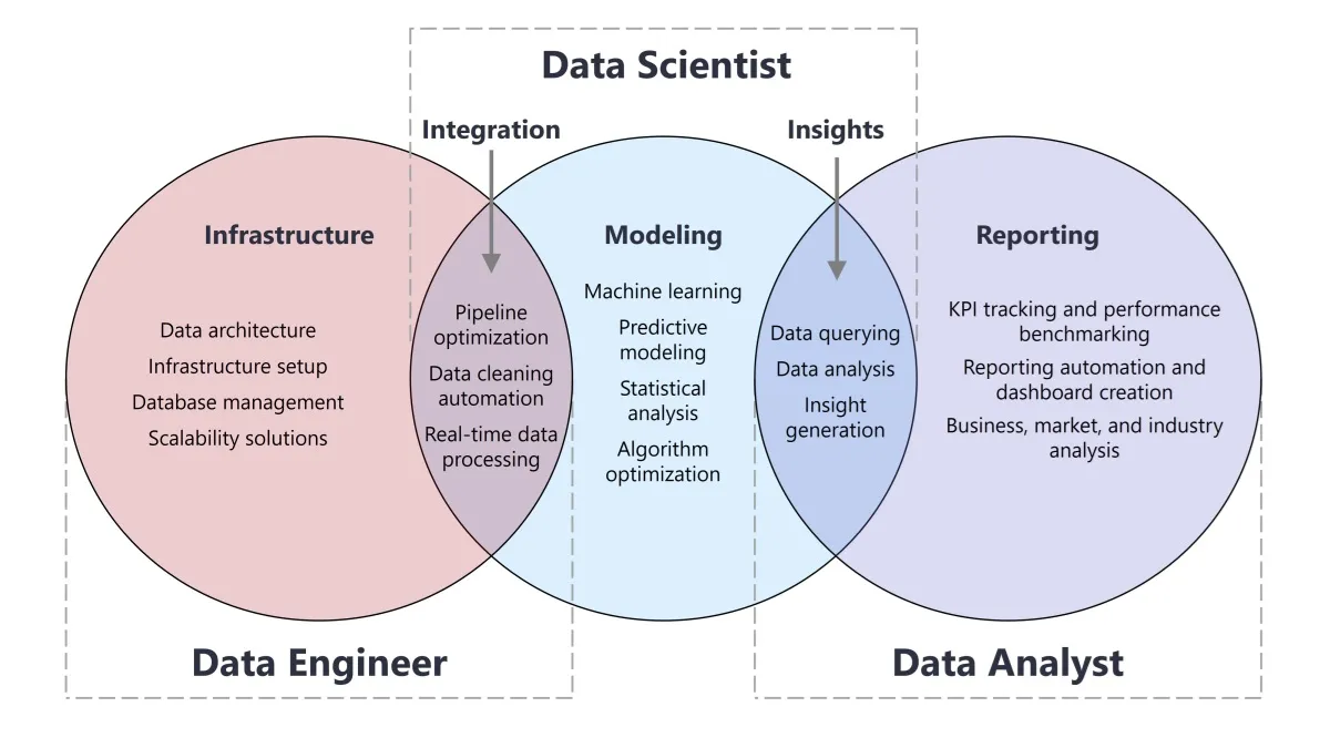
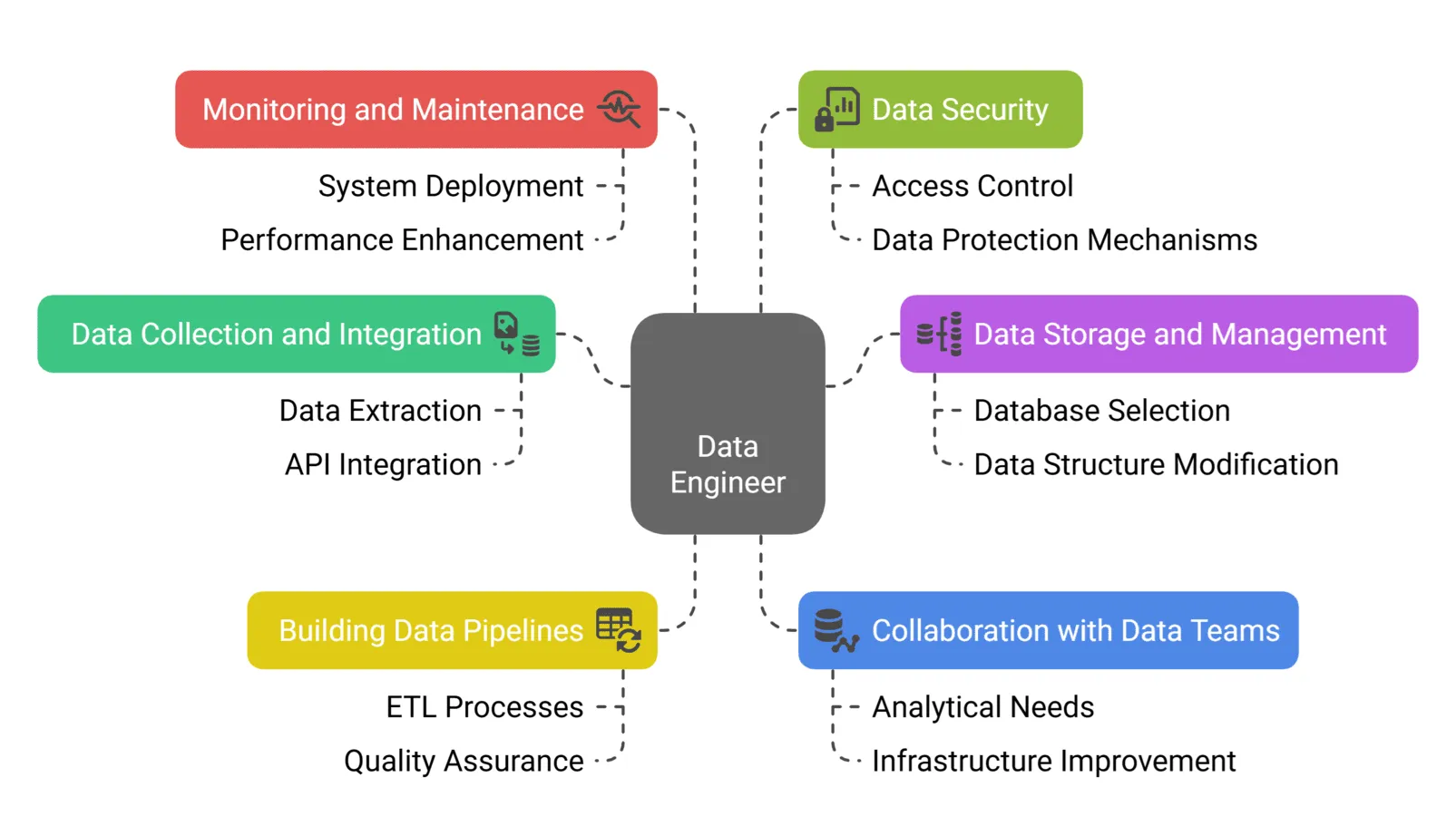 Data Engineer Responsibilities Illustrated!
Core Concepts
What is Data Engineering?
Data engineering is the discipline of designing infrastructure that collects, stores, and processes data. It involves:
- Building data pipelines that move data from sources to destinations
- Implementing ETL/ELT processes for data transformation
- Managing data quality through validation and governance
- Ensuring scalability to handle growing data volumes
- Maintaining data security and compliance with regulations
Key Roles and Responsibilities
Data engineers are responsible for:
- Pipeline Development: Creating automated workflows for data extraction, transformation, and loading
- Data Integration: Consolidating data from disparate sources into unified systems
- Performance Optimization: Ensuring pipelines operate efficiently at scale
- Data Quality Assurance: Implementing validation rules and data integrity checks
- Infrastructure Management: Maintaining cloud-based or on-premises data platforms
- Collaboration: Working with data scientists, analysts, and business stakeholders
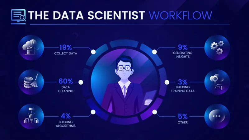 Data Scientist Workflow Illustrated
Data Pipeline Architectures
Understanding Data Pipelines
A data pipeline is a system that moves data from one place to another. Pipelines connect data sources (CRM platforms, databases, event logs) to destinations (data warehouses, databases, or centralized locations). They can include multiple branches, loops, and processes.
ETL vs ELT: Core Differences
ETL (Extract, Transform, Load)
ETL is a sequential process where transformation occurs before loading data into the destination.
Process Flow:
- Extract: Data is extracted from multiple heterogeneous sources (databases, CRM systems, flat files, APIs)
- Transform: Data undergoes cleaning, standardization, enrichment, aggregation, and validation
- Load: Transformed data is loaded into the target system (data warehouse or database)
Characteristics:
- Transformation happens in-memory or in a separate transformation engine
- Data is processed and cleaned before reaching the destination
- Suitable for structured data environments where data quality is critical
- Ideal for batch processing scenarios and historical data analysis
- More expensive to write due to multiple layers of encoding and compression
Use Cases:
- Traditional data warehousing applications
- Scenarios requiring strict data quality before storage
- On-premises systems with limited destination compute power
- Compliance-heavy industries (finance, healthcare)
ELT (Extract, Load, Transform)
ELT loads raw data into the destination before applying transformations.
Process Flow:
- Extract: Data is extracted from source systems
- Load: Raw data is loaded directly into the target storage (data lake or cloud data warehouse)
- Transform: Transformation occurs within the destination system using its compute resources
Characteristics:
- Leverages the processing power of modern cloud data warehouses
- All data is available in the destination for flexible transformation
- Faster initial data loading with reduced latency
- Transformation is deferred until needed for specific use cases
- Scales well with cloud-based infrastructure
Use Cases:
- Cloud-based data platforms (Snowflake, BigQuery, Redshift)
- Big data applications requiring flexible schemas
- Real-time analytics and streaming data
- Data science and exploratory analysis
- Scenarios requiring access to raw data
Comparison Summary
| Aspect | ETL | ELT |
|---|---|---|
| Transformation Timing | Before loading | After loading |
| Processing Location | External transformation engine | Within destination system |
| Data Storage | Only transformed data stored | Raw + transformed data stored |
| Flexibility | Less flexible, predefined transformations | More flexible, transform as needed |
| Performance | Dependent on transformation engine | Leverages destination compute power |
| Cost | Higher transformation costs | Lower transformation costs, higher storage |
| Best For | Structured data, compliance-heavy | Big data, cloud platforms, ML workloads |
Hybrid and Advanced Patterns
ELTL (Extract, Load, Transform, Load)
A variation where data is:
- Extracted from sources
- Loaded into low-cost storage (data lake)
- Transformed to conform to a data warehouse model
- Loaded into a cloud data warehouse staging area
This approach is useful when you have diverse data sources for different purposes, establishing both a data lake for discovery and a traditional data warehouse for structured analytics.
Real-Time Streaming Pipelines
Unlike batch-based ETL or ELT, streaming pipelines process data as it arrives using technologies like:
- Apache Kafka: Distributed event streaming platform
- Apache Spark Streaming: Real-time data processing
- AWS Kinesis: Cloud-based streaming service
Streaming enables immediate insights and actions for use cases like fraud detection, IoT monitoring, and real-time recommendations.
Reverse ETL
Reverse ETL flows data from data warehouses back to operational systems (CRMs, marketing platforms) to activate insights. The transformation step converts warehouse formats to align with target system requirements.
Pipeline Components
Control Flow
Ensures orderly processing of tasks with precedence constraints. Controls the sequence of operations and handles outcomes (success, failure, completion) before initiating subsequent tasks.
Data Flow
Within each task, data flows from source through transformations to destination. Includes operations like:
- Data extraction and parsing
- Validation and cleansing
- Enrichment and joining
- Aggregation and filtering
- Format conversion
Data Modeling
Dimensional Modeling Fundamentals
Dimensional modeling is a design technique optimized for querying and analysis in data warehouses. It organizes data into fact tables and dimension tables to support intuitive business analysis.
Fact Tables
- Store measurable events or transactions (sales, clicks, orders)
- Contain metrics (quantities, amounts, counts) and foreign keys to dimensions
- Typically denormalized for query performance
- Form the center of star or snowflake schemas
Example metrics:
revenue,quantity_sold,order_count,clicks,conversion_rate
Dimension Tables
- Provide context and attributes for facts (who, what, when, where, why)
- Contain descriptive information used for filtering and grouping
- Connected to fact tables via foreign keys
- Represent different perspectives of data (time, product, customer, location)
Common dimensions:
- Time/Date, Customer, Product, Geography, Employee, Store
Schema Patterns
Star Schema
The star schema is the simplest dimensional model, featuring a central fact table surrounded by denormalized dimension tables.
Structure:
1
2
3
4
5
        [Time Dimension]
              |
[Product]--[Fact Table]--[Customer]
              |
        [Location Dimension]
Characteristics:
- Denormalized dimensions: All attributes in single tables
- Direct relationships: Dimensions connect directly to fact table
- Simple queries: Minimal joins required (fact + dimensions)
- Fast performance: Optimized for query speed
- Redundant data: Repeated values in dimension tables
Advantages:
- Faster query execution due to fewer joins
- Simpler to understand and navigate
- Easier to implement and set up
- Ideal for business intelligence and reporting
- Better performance for dashboards
Disadvantages:
- Higher storage requirements due to denormalization
- Data redundancy in dimension tables
- More difficult to maintain data integrity
- Update anomalies when changing dimensional data
Use Cases:
- Small to medium datasets
- Real-time analytics and dashboards
- Scenarios prioritizing query speed over storage
- Business intelligence applications
- Limited dimensional hierarchies
Snowflake Schema
The snowflake schema normalizes dimension tables into multiple related tables, creating a structure that resembles a snowflake.
Structure:
1
2
3
4
5
6
7
    [Category]
        |
    [Subcategory]
        |
    [Product]--[Fact Table]--[Customer]
                    |
            [City]--[State]--[Country]
Characteristics:
- Normalized dimensions: Split into hierarchical tables
- Reduced redundancy: Data stored once in appropriate tables
- Complex queries: More joins required to traverse hierarchies
- Smaller storage footprint: Less data duplication
- Better data integrity: Easier to maintain consistency
Advantages:
- Storage efficiency through normalization
- Reduced data redundancy and update anomalies
- Better data integrity and consistency
- Easier to maintain complex hierarchies
- Supports slowly changing dimensions (SCD)
Disadvantages:
- Slower query performance due to multiple joins
- More complex query design
- Harder for business users to understand
- Increased query complexity for BI tools
Use Cases:
- Large, normalized datasets with deep hierarchies
- Systems requiring frequent updates
- Organizations prioritizing storage efficiency
- Complex dimension structures (multi-level categories)
- Enterprise data warehouses with strict governance
Comparison Matrix
| Feature | Star Schema | Snowflake Schema |
|---|---|---|
| Structure | Denormalized | Normalized |
| Dimension Tables | Single level | Multiple levels |
| Query Complexity | Simple | Complex |
| Query Performance | Faster | Slower |
| Storage Space | More | Less |
| Data Redundancy | High | Low |
| Maintenance | Harder | Easier |
| Data Integrity | Lower | Higher |
| Setup Difficulty | Easy | Moderate |
Modern Cloud Considerations
With cloud data warehouses (Snowflake, BigQuery, Redshift), the traditional performance boundaries are dissolving:
- Computational power makes join performance less critical
- Storage is cheap, reducing the advantage of normalization
- Hybrid approaches are common: denormalize frequently-used dimensions, normalize hierarchical or high-cardinality dimensions
- Query optimization and caching reduce the performance gap
Many data teams use a pragmatic approach:
- Denormalize for speed: Dimensions used constantly (time, core product/customer attributes)
- Normalize for flexibility: Deep hierarchies, frequently changing dimensions (org charts, geographies)
File Formats for Data Engineering
Efficient data storage formats are critical for performance and cost optimization in data engineering. Different formats offer trade-offs between read/write speed, storage efficiency, and feature richness.
CSV (Comma-Separated Values)
Characteristics:
- Text-based, human-readable format
- Simple structure with rows and columns
- Universal compatibility across tools
- No compression or optimization
Performance:
- Slowest read/write operations
- Largest file sizes (2-4x larger than binary formats)
- High memory usage during operations
- No columnar access or predicate pushdown
Use Cases:
- Data exchange with non-technical users
- Simple data exports and imports
- Systems requiring human readability
- Small datasets where performance isn’t critical
Avoid When:
- Working with large datasets (>100MB)
- Performance is a priority
- Storage costs are a concern
Parquet
Characteristics:
- Columnar storage format optimized for analytics
- Built on Apache Arrow specification
- Industry-standard for big data ecosystems
- Multiple layers of encoding and compression
Storage Features:
- Dictionary encoding: Efficient storage of repeated values
- Run-length encoding (RLE): Compresses consecutive identical values
- Data page compression: Additional compression (Snappy, Gzip, Brotli, LZ4, Zstd)
- Typically 3-10x smaller than CSV files
Performance:
- Efficient for read-heavy workloads
- Supports columnar access (read specific columns only)
- Predicate pushdown: Filter data at storage level
- More expensive to write than Feather
- Excellent for analytical queries and aggregations
Compatibility:
- Supported by: Spark, Hive, Impala, Presto, BigQuery, Redshift, Snowflake
- Works across multiple languages (Python, Java, Scala, R)
- Standard format for data lakes and warehouses
Use Cases:
- Long-term data storage in data lakes
- Analytics workloads with complex queries
- Big data processing with Spark/Hadoop
- Data warehousing and BI applications
- Multi-system data sharing
Code Example:
1
2
3
4
5
6
7
8
import pandas as pd
import pyarrow.parquet as pq

# Write with compression
df.to_parquet('data.parquet', compression='snappy')

# Read specific columns
df = pd.read_parquet('data.parquet', columns=['col1', 'col2'])
Feather
Characteristics:
- Binary columnar format based on Apache Arrow
- Designed for speed and interoperability
- Minimal encoding (raw columnar Arrow memory)
- Lightweight and fast
Performance:
- Fastest read/write speeds among common formats (2-20x faster than CSV)
- Lowest memory usage during operations
- Unmodified raw columnar structure
- Optimized for temporary storage and inter-process communication
Storage:
- Moderate file sizes (between CSV and Parquet)
- Optional compression (LZ4, Zstd)
- Less compression than Parquet due to simpler encoding
Compatibility:
- Native support in Pandas and Arrow
- Language-agnostic (Python, R, Julia)
- IPC (Inter-Process Communication) for data sharing
Use Cases:
- Short-term/ephemeral storage
- Fast data transfer between processes
- Caching intermediate results
- Data exchange between Python and R
- When speed is the primary concern
- Temporary analytical workloads
Limitations:
- Less feature-rich than Parquet
- Not optimal for long-term archival
- Larger file sizes than highly compressed Parquet
Code Example:
1
2
3
4
5
6
7
8
import pandas as pd
import pyarrow.feather as feather

# Write with compression
df.to_feather('data.feather', compression='zstd')

# Read
df = pd.read_feather('data.feather')
Format Selection Guidelines
Choose CSV When:
- Human readability is required
- Maximum compatibility is needed
- Dataset is very small (<10MB)
- One-time data exchange
Choose Parquet When:
- Data will be stored long-term
- Analytics and BI queries are primary use case
- Working with big data systems (Spark, Hive)
- Storage efficiency is important
- Multiple systems need to access data
- Complex queries with column selection
Choose Feather When:
- Speed is the top priority
- Temporary storage or caching
- Sharing data between Python and R
- Inter-process communication
- Low memory usage is critical
- Rapid prototyping and development
Performance Benchmarks (5M Records)
| Format | Write Time | Read Time | File Size | Compression |
|---|---|---|---|---|
| CSV | 25 seconds | 15 seconds | 330 MB | None |
| Feather | 3.98 seconds | 2.3 seconds | 140 MB | Optional |
| Parquet (Snappy) | 8 seconds | 4 seconds | 140 MB | Snappy |
| Parquet (Gzip) | 15 seconds | 6 seconds | 80 MB | Gzip |
| Parquet (Zstd) | 12 seconds | 5 seconds | 70 MB | Zstd |
Key Insights:
- Feather is fastest for read/write operations
- Parquet with Zstd compression offers best storage efficiency
- CSV is 10-25x slower than binary formats
- Parquet is ideal for analytics; Feather for rapid data access
Additional Formats
ORC (Optimized Row Columnar)
- Columnar format like Parquet
- Optimized for Hadoop/Hive ecosystems
- Used by Facebook and large institutions
- Better for Hive-based workflows
HDF5 (Hierarchical Data Format)
- Self-describing format
- Stores mixed objects (arrays, metadata, groups)
- Good for scientific computing
- More complex than Parquet/Feather
API Integration Patterns
APIs enable data engineers to extract data from various sources and integrate disparate systems. Understanding different API architectures is crucial for effective data pipeline design.
REST APIs
REST (Representational State Transfer) is the most common API architecture, using HTTP methods to interact with resources.
Core Principles
Resource-Based Architecture:
- Each resource has a unique identifier (URI)
- Resources represent data or objects (users, posts, orders)
- Standard HTTP methods operate on resources
HTTP Methods:
GET: Retrieve dataPOST: Create new resourcesPUT/PATCH: Update existing resourcesDELETE: Remove resources
Response Formats:
- JSON (most common)
- XML
- HTML
Characteristics:
- Fixed structure: Endpoints return predefined datasets
- Multiple requests: Often need separate calls for related data
- Stateless: Each request is independent
- Cacheable: Supports HTTP caching mechanisms
- Mature tooling: Extensive documentation, OpenAPI/Swagger support
Advantages
- Simple and widely understood
- Excellent tooling and documentation
- Easy to implement and debug
- Industry standard for integrations
- Works well with HTTP infrastructure (load balancers, proxies)
Disadvantages
- Over-fetching: Returns more data than needed
- Under-fetching: Requires multiple requests for related data
- N+1 problem: Multiple round trips for nested relationships
- Fixed structure: Less flexible for varying client needs
- API versioning: Breaking changes require version management
REST in Data Engineering
Use Cases:
- Extracting data from third-party services (Salesforce, Stripe, Shopify)
- Webhook integrations for event-driven pipelines
- Batch data extraction for ETL processes
- Public API consumption
Best Practices:
- Implement retry logic with exponential backoff
- Use pagination for large datasets
- Apply rate limiting to avoid throttling
- Cache responses when appropriate
- Handle errors gracefully with proper logging
Example ETL Pattern:
1
2
3
4
5
6
7
8
9
10
11
12
13
14
15
16
17
18
19
20
21
22
23
import requests
import time

def fetch_paginated_data(base_url, params):
    all_data = []
    page = 1

    while True:
        params['page'] = page
        response = requests.get(base_url, params=params)

        if response.status_code == 429:  # Rate limited
            time.sleep(60)
            continue

        data = response.json()
        if not data:
            break

        all_data.extend(data)
        page += 1

    return all_data
GraphQL APIs
GraphQL is a query language and runtime that allows clients to request exactly the data they need from APIs.
Core Concepts
Schema-Defined:
- Strong typing system defines available data
- Self-documenting with introspection
- Single endpoint for all queries
Query Language:
- Clients specify exact fields needed
- Nested queries fetch related data in one request
- Queries mirror UI structure
Operations:
- Queries: Fetch data (equivalent to GET)
- Mutations: Modify data (equivalent to POST/PUT/DELETE)
- Subscriptions: Real-time updates via WebSockets
Characteristics
- Flexible data fetching: Request only what you need
- Single request: Avoid multiple round trips
- Type safety: Strongly typed schema
- Evolving APIs: Add fields without breaking changes
- Nested relationships: Fetch related data efficiently
Advantages
- Eliminates over-fetching and under-fetching
- Reduces number of API calls (lower latency)
- Better performance for complex data requirements
- Self-documenting with schema introspection
- Ideal for frontend-driven applications
- Versioning not required (additive changes)
Disadvantages
- Steeper learning curve for developers
- More complex to implement on server side
- Caching is more challenging than REST
- Potential for expensive queries (query depth limits needed)
- Less mature tooling for some use cases
- Requires understanding of graph structure
GraphQL in Data Engineering
Use Cases:
- Extracting complex nested data from APIs (GitHub, Shopify, Contentful)
- Reducing API calls in data pipelines
- Flexible data extraction for exploratory analysis
- Wrapping multiple REST APIs into unified interface
Data Pipeline Benefits:
- Fetch exactly needed fields (reduce bandwidth)
- Combine multiple related resources in one query
- Lower network latency with fewer requests
Example ETL Pattern:
1
2
3
4
5
6
7
8
9
10
11
12
13
14
15
16
17
18
19
20
21
22
23
24
25
26
import requests

query = """
query {
  users(first: 100) {
    nodes {
      id
      name
      email
      orders {
        id
        total
        createdAt
      }
    }
  }
}
"""

response = requests.post(
    'https://api.example.com/graphql',
    json={'query': query},
    headers={'Authorization': f'Bearer {token}'}
)

data = response.json()['data']['users']['nodes']
REST vs GraphQL Comparison
| Aspect | REST | GraphQL |
|---|---|---|
| Architecture | Multiple endpoints | Single endpoint |
| Data Fetching | Fixed structure | Client-specified fields |
| Over-fetching | Common | Eliminated |
| Under-fetching | Multiple requests | Single request |
| Versioning | Required (v1, v2) | Not required |
| Caching | HTTP caching | Custom caching |
| Learning Curve | Simple | Moderate |
| Tooling | Mature (Postman, Swagger) | Growing (GraphiQL) |
| Network Calls | Multiple for related data | Single for nested data |
| Use Case | Simple CRUD, standard APIs | Complex data needs, mobile apps |
Hybrid Approaches
GraphQL Wrapper Over REST
Organizations can create a GraphQL layer on top of existing REST APIs to modernize interactions without complete rewrites. The GraphQL server acts as a facade, translating GraphQL queries into REST API calls.
Benefits:
- Leverage existing REST APIs
- Provide GraphQL benefits to clients
- Gradual migration path
- Unified API for multiple backends
REST Wrapper Over GraphQL
Conversely, organizations can expose GraphQL APIs as REST endpoints for external integrations that expect RESTful interfaces.
Benefits:
- Maintain single source of truth (GraphQL)
- Support legacy integrations
- Auto-generate REST documentation (OpenAPI)
- Simplify external developer experience
API Integration Best Practices
- Implement Robust Error Handling: Retry transient failures, handle rate limits, log errors
- Use Pagination: Handle large datasets efficiently
- Respect Rate Limits: Implement backoff strategies
- Secure Credentials: Use secrets managers, never hardcode API keys
- Monitor API Usage: Track latency, error rates, quota consumption
- Version Your Integrations: Handle API versioning changes
- Cache Appropriately: Reduce unnecessary API calls
- Validate Responses: Check data quality and schema compliance
Data Storage Architectures
Modern organizations require storage systems that balance performance, scalability, cost, and flexibility. Three primary architectures have emerged: data warehouses, data lakes, and data lakehouses.
Data Warehouse
Definition: A centralized repository optimized for storing, managing, and analyzing structured data from multiple sources.
Architecture
- Schema-on-Write: Data is transformed and structured before loading
- Optimized for queries: Indexed, partitioned, and aggregated for fast analytics
- Columnar storage: Stores data by columns for efficient aggregation
- OLAP (Online Analytical Processing): Designed for complex analytical queries
Characteristics
- Stores cleansed, transformed, and structured data
- Enforces strict schemas and data types
- Provides high query performance for BI and reporting
- Supports concurrent users with low latency
- Includes metadata, indexing, and optimization layers
Technologies
- Cloud: Snowflake, Google BigQuery, Amazon Redshift, Azure Synapse Analytics
- Traditional: Teradata, Oracle, IBM Db2 Warehouse
- Open Source: Apache Hive, Greenplum
Advantages
- Fast query performance: Optimized for analytics and BI
- Data quality: Enforced schemas and validation
- Consistency: ACID transactions ensure reliability
- Mature tools: Extensive BI tool integration
- Governance: Built-in security and compliance features
Disadvantages
- Limited flexibility: Difficult to handle unstructured data
- Schema changes: Costly to modify structures
- Storage costs: Can be expensive at scale
- ETL complexity: Requires upfront data modeling
- Limited ML support: Proprietary formats may not support ML tools
Use Cases
- Business intelligence and reporting
- Historical trend analysis
- Regulatory compliance and auditing
- Financial reporting
- Sales and marketing analytics
- Enterprise dashboards
Data Lake
Definition: A centralized repository that stores raw data in its native format (structured, semi-structured, and unstructured) at scale.
Architecture
- Schema-on-Read: Data is structured when accessed, not when stored
- Object storage: Stores files in distributed systems (S3, ADLS, GCS)
- Flexible formats: Supports JSON, XML, CSV, Parquet, images, videos, logs
- Horizontal scalability: Easily scales to petabytes
Characteristics
- Stores all types of data: structured, semi-structured, unstructured
- No predefined schema required
- Low-cost storage using commodity hardware or cloud object storage
- Data is kept in raw form for flexibility
- Optimized for data science and machine learning
Technologies
- Cloud: Amazon S3, Azure Data Lake Storage (ADLS), Google Cloud Storage (GCS)
- Frameworks: Hadoop HDFS, Apache Spark
- Query engines: Presto, Apache Drill, Athena
Advantages
- Cost-effective: Low-cost storage for large volumes
- Flexibility: Store any data type without transformation
- Scalability: Easily scales to petabytes and beyond
- ML/AI support: Native formats work with Python, TensorFlow, PyTorch
- Exploratory analysis: Supports data discovery and experimentation
Disadvantages
- Data swamps: Can become unmanaged and difficult to navigate
- No ACID guarantees: Lacks transactional consistency
- Slow queries: Scanning large files is inefficient
- Limited governance: Weaker security and compliance controls
- Complexity: Requires skilled data engineers to manage
- Quality issues: Raw data may contain errors and inconsistencies
Use Cases
- Machine learning and AI workloads
- Data science experimentation
- Archival and long-term storage
- IoT and sensor data collection
- Log aggregation and analysis
- Real-time streaming data landing zone
Data Lakehouse
Definition: A hybrid architecture that combines the flexibility and scale of data lakes with the governance and performance of data warehouses.
Architecture
- Unified platform: Single system for all data types and workloads
- Open table formats: Delta Lake, Apache Iceberg, Apache Hudi
- ACID transactions: Ensures data consistency and reliability
- Metadata layer: Tracks schemas, lineage, and data quality
- Separation of storage and compute: Independent scaling
Key Components
1. Ingestion Layer
- Collects data from sources (databases, APIs, streams, files)
- Supports batch and real-time ingestion
- Maintains data lineage from source to destination
2. Storage Layer
- Object storage (S3, ADLS, GCS) for cost-efficiency
- Open formats (Parquet, ORC) for broad compatibility
- Decoupled from compute for independent scaling
3. Metadata Layer
- Catalogs and indexes all datasets
- Tracks schemas, versions, and lineage
- Enables data discovery and governance
4. Processing Layer
- Apache Spark, Databricks, Snowflake for transformations
- Supports SQL, Python, Scala, R
- Handles batch and streaming workloads
5. Consumption Layer
- BI tools (Tableau, Power BI, Looker)
- ML frameworks (TensorFlow, PyTorch, scikit-learn)
- Direct data access via APIs and notebooks
Characteristics
- Unified governance: Single metadata layer for all data
- ACID compliance: Reliable transactions across all operations
- Schema enforcement and evolution: Flexible yet structured
- Multi-workload support: BI, ML, real-time analytics in one platform
- Time travel: Access historical data versions
- Data lineage: End-to-end tracking of data transformations
Technologies
- Platforms: Databricks, Snowflake (with Iceberg), Google BigQuery
- Table formats: Delta Lake, Apache Iceberg, Apache Hudi
- Query engines: Spark SQL, Presto, Trino
- Governance: Unity Catalog, AWS Glue Data Catalog
Advantages
- Unified platform: No need for separate lake and warehouse
- Cost-effective: Low-cost storage with on-demand compute
- Flexibility: Handles all data types (structured, semi-structured, unstructured)
- Performance: Optimized for analytics with indexing and caching
- Open standards: Avoids vendor lock-in with open formats
- Real-time capabilities: Supports streaming and batch workloads
- ML/AI support: Direct access for data science tools
Disadvantages
- Complexity: Requires understanding of multiple technologies
- Maturity: Newer architecture with evolving best practices
- Migration effort: Transitioning from existing systems can be challenging
- Skillset requirements: Demands expertise in modern data platforms
Use Cases
- Organizations needing both BI and ML on same data
- Real-time analytics and streaming workloads
- Unified governance across all data
- Companies modernizing legacy data warehouses
- Multi-cloud or hybrid cloud strategies
- Advanced analytics with diverse data types
Comparative Analysis
| Feature | Data Warehouse | Data Lake | Data Lakehouse |
|---|---|---|---|
| Data Types | Structured | All types | All types |
| Schema | Schema-on-write | Schema-on-read | Both |
| Cost | High | Low | Moderate |
| Performance | Fast (optimized) | Slow (raw scans) | Fast (optimized) |
| Flexibility | Low | High | High |
| ACID Support | Yes | No | Yes |
| Governance | Strong | Weak | Strong |
| Use Cases | BI, reporting | ML, exploration | BI + ML unified |
| Data Quality | High | Variable | High (with enforcement) |
| Scalability | Moderate-High | Very High | Very High |
| Query Latency | Low | High | Low-Moderate |
Choosing the Right Architecture
Choose Data Warehouse When:
- Primary use case is BI and reporting
- Data is mostly structured
- Query performance is critical
- Strong governance and compliance required
- Users need low-latency dashboards
Choose Data Lake When:
- Storing diverse, unstructured data
- Primary use case is ML and data science
- Cost optimization is priority
- Exploratory analysis and experimentation
- Long-term archival storage
Choose Data Lakehouse When:
- Need both BI and ML workloads
- Require unified governance
- Want to avoid data duplication
- Real-time analytics required
- Modernizing from legacy systems
- Multi-workload support (batch, streaming, ML)
Medallion Architecture in Lakehouses
A common design pattern in data lakehouses is the medallion architecture, which organizes data into layers:
Bronze Layer (Raw)
- Landing zone for raw data from sources
- Minimal transformation (perhaps schema validation)
- Data stored as-is for auditing and reprocessing
Silver Layer (Refined)
- Cleaned and validated data
- Deduplicated, filtered, and standardized
- Conformed to business rules
- Enriched with additional context
Gold Layer (Curated)
- Business-level aggregates and features
- Optimized for specific use cases (BI, ML)
- Pre-joined tables for performance
- Production-ready datasets
Benefits:
- Clear data quality progression
- Reusable transformation logic
- Easy debugging and data lineage
- Separation of concerns
Best Practices
Pipeline Design and Development
1. Idempotency and Reproducibility
Principle: Pipelines should produce the same results when run multiple times with the same inputs.
Implementation:
- Use deterministic transformations
- Avoid relying on system time or random values
- Implement checkpointing and state management
- Use versioning for code and data schemas
Example Pattern:
1
2
3
4
5
6
7
8
def process_data(input_path, output_path, run_date):
    # Use run_date instead of datetime.now()
    df = read_data(input_path)
    df['processing_date'] = run_date
    df = transform(df)

    # Overwrite mode ensures idempotency
    df.write.mode('overwrite').parquet(output_path)
2. Incremental Processing
Principle: Process only new or changed data rather than reprocessing entire datasets.
Strategies:
- Timestamp-based: Track
last_updatedorcreated_atfields - Change Data Capture (CDC): Capture database changes at source
- Watermarking: Track last successfully processed record
- Partitioning: Process data by date/time partitions
Benefits:
- Reduced processing time and costs
- Lower resource consumption
- Faster pipeline execution
- Better scalability
Example:
1
2
3
4
5
6
7
8
9
10
11
# Track last processed timestamp
last_run = get_last_watermark()

# Only fetch new records
new_data = spark.read \
    .option("query", f"SELECT * FROM table WHERE updated_at > '{last_run}'") \
    .jdbc(url, table, properties)

# Process and update watermark
process_data(new_data)
update_watermark(current_timestamp)
3. Data Quality Checks
Principle: Validate data at every stage to maintain integrity and reliability.
Validation Layers:
Source Validation:
- Schema validation (correct columns and types)
- Null checks on required fields
- Range and format validation
- Referential integrity
Transformation Validation:
- Row count consistency
- Aggregation checks
- Business rule validation
- Duplicate detection
Destination Validation:
- Completeness checks
- Freshness monitoring
- Accuracy verification
Implementation Example:
1
2
3
4
5
6
7
8
9
10
11
12
13
14
15
16
17
18
19
20
21
def validate_data(df):
    validations = []

    # Check for nulls in required fields
    null_check = df.filter(df['id'].isNull()).count()
    validations.append(('null_check', null_check == 0))

    # Check value ranges
    range_check = df.filter((df['age'] < 0) | (df['age'] > 120)).count()
    validations.append(('range_check', range_check == 0))

    # Check duplicates
    duplicate_check = df.count() == df.distinct().count()
    validations.append(('duplicate_check', duplicate_check))

    # Raise alert if any validation fails
    for check_name, passed in validations:
        if not passed:
            raise DataQualityException(f"{check_name} failed")

    return df
4. Error Handling and Retry Logic
Principle: Build resilient pipelines that gracefully handle failures.
Strategies:
- Exponential backoff: Increase wait time between retries
- Circuit breakers: Stop retrying after threshold failures
- Dead letter queues: Store failed records for manual review
- Alerting: Notify on-call engineers of critical failures
Example Pattern:
1
2
3
4
5
6
7
8
9
10
11
12
13
14
15
16
17
18
19
20
21
22
23
24
import time
from functools import wraps

def retry_with_backoff(max_retries=3, backoff_factor=2):
    def decorator(func):
        @wraps(func)
        def wrapper(*args, **kwargs):
            for attempt in range(max_retries):
                try:
                    return func(*args, **kwargs)
                except TransientError as e:
                    if attempt == max_retries - 1:
                        raise
                    wait_time = backoff_factor ** attempt
                    print(f"Retry {attempt + 1}/{max_retries} after {wait_time}s")
                    time.sleep(wait_time)
        return wrapper
    return decorator

@retry_with_backoff(max_retries=3)
def fetch_api_data(url):
    response = requests.get(url)
    response.raise_for_status()
    return response.json()
5. Monitoring and Observability
Principle: Track pipeline health, performance, and data quality continuously.
Key Metrics:
- Pipeline metrics: Runtime, success/failure rate, throughput
- Data metrics: Row counts, data freshness, schema changes
- Infrastructure metrics: CPU, memory, network I/O
- Business metrics: SLA compliance, data latency
Monitoring Tools:
- Logging: Structured logs with correlation IDs
- Metrics: Prometheus, CloudWatch, Datadog
- Alerting: PagerDuty, Opsgenie, Slack notifications
- Dashboards: Grafana, Kibana, custom BI dashboards
Implementation:
1
2
3
4
5
6
7
8
9
10
11
12
13
14
15
16
17
18
19
20
21
22
23
24
25
26
27
28
29
30
31
32
33
34
35
36
37
38
39
40
41
42
import logging
from datetime import datetime

logger = logging.getLogger(__name__)

def pipeline_with_monitoring(pipeline_name):
    start_time = datetime.now()
    record_count = 0

    try:
        logger.info(f"Starting pipeline: {pipeline_name}")

        # Execute pipeline
        df = extract_data()
        record_count = df.count()
        df = transform_data(df)
        load_data(df)

        duration = (datetime.now() - start_time).total_seconds()

        # Log success metrics
        logger.info(f"Pipeline completed: {pipeline_name}", extra={
            'duration_seconds': duration,
            'records_processed': record_count,
            'status': 'success'
        })

        # Send metrics to monitoring system
        send_metric('pipeline.duration', duration, tags={'pipeline': pipeline_name})
        send_metric('pipeline.records', record_count, tags={'pipeline': pipeline_name})

    except Exception as e:
        duration = (datetime.now() - start_time).total_seconds()
        logger.error(f"Pipeline failed: {pipeline_name}", extra={
            'duration_seconds': duration,
            'error': str(e),
            'status': 'failed'
        })

        # Alert on failure
        send_alert(f"Pipeline {pipeline_name} failed: {str(e)}")
        raise
Data Modeling Best Practices
1. Start with Business Requirements
- Understand key metrics and dimensions before designing schemas
- Collaborate with business stakeholders and analysts
- Document business logic and definitions
- Align models with reporting and analytical needs
2. Balance Normalization and Performance
- Normalize to reduce redundancy and improve data integrity
- Denormalize for query performance when needed
- Use hybrid approaches in cloud warehouses
- Profile queries to identify bottlenecks
3. Design for Change
- Slowly Changing Dimensions (SCD): Track historical changes
- Type 1: Overwrite (no history)
- Type 2: Add new row with versioning (full history)
- Type 3: Add columns for previous values (limited history)
- Version schemas to handle evolution
- Use additive changes when possible
- Implement graceful schema migration strategies
SCD Type 2 Example:
1
2
3
4
5
6
7
8
9
10
CREATE TABLE dim_customer (
    customer_key INT PRIMARY KEY,      -- Surrogate key
    customer_id VARCHAR(50),           -- Natural key
    customer_name VARCHAR(200),
    email VARCHAR(200),
    address VARCHAR(500),
    valid_from DATE,                   -- Effective date
    valid_to DATE,                     -- Expiration date
    is_current BOOLEAN                 -- Current record flag
);
4. Use Surrogate Keys
- Generate surrogate keys (auto-increment or UUIDs) for dimension tables
- Separate business keys from technical keys
- Simplifies updates and maintains referential integrity
- Improves join performance with integer keys
5. Partition Large Tables
- Partition by date/time for time-series data
- Reduces scan volumes for queries
- Improves query performance and reduces costs
- Enables efficient data retention policies
Example:
1
2
3
4
5
6
7
8
CREATE TABLE fact_sales (
    sale_id BIGINT,
    product_key INT,
    customer_key INT,
    sale_date DATE,
    amount DECIMAL(10,2)
)
PARTITION BY RANGE (sale_date);
Performance Optimization
1. Optimize File Sizes
Problem: Too many small files or very large files degrade performance.
Guidelines:
- Target file sizes: 128MB - 1GB for Parquet
- Use coalescing or repartitioning to optimize file counts
- Configure appropriate compression (Snappy for speed, Zstd for size)
Example:
1
2
# Optimize file sizes before writing
df.repartition(10).write.parquet('output/', compression='snappy')
2. Predicate Pushdown and Column Pruning
Principle: Filter and select data as early as possible in the pipeline.
Techniques:
- Predicate pushdown: Apply filters at data source
- Column pruning: Read only required columns
- Partition pruning: Skip irrelevant partitions
Example:
1
2
3
4
5
6
7
8
9
# Good: Filter pushed to storage layer
df = spark.read.parquet('data/') \
    .select('id', 'name', 'amount') \
    .filter(col('date') >= '2024-01-01')

# Bad: Read entire dataset then filter
df = spark.read.parquet('data/')
df = df.select('id', 'name', 'amount')
df = df.filter(col('date') >= '2024-01-01')
3. Efficient Joins
Strategies:
- Broadcast joins: Broadcast small tables to all nodes
- Sort-merge joins: Sort both tables before joining
- Bucketing: Pre-partition data on join keys
- Filter before joining: Reduce data volumes
Example:
1
2
3
4
5
6
7
8
from pyspark.sql.functions import broadcast

# Broadcast small dimension table
result = fact_df.join(
    broadcast(dim_df),
    on='product_id',
    how='inner'
)
4. Caching and Materialization
When to cache:
- Datasets used multiple times in same pipeline
- Expensive computations reused across queries
- Iterative algorithms (ML training)
Caution:
- Don’t cache everything (memory constraints)
- Clear cache when no longer needed
- Monitor memory usage
Example:
1
2
3
4
5
6
7
8
9
# Cache for reuse
df_clean = df.filter(col('valid') == True).cache()

# Use multiple times
summary1 = df_clean.groupBy('category').count()
summary2 = df_clean.groupBy('region').sum('amount')

# Clear when done
df_clean.unpersist()
Security and Governance
1. Data Access Control
- Implement role-based access control (RBAC)
- Use fine-grained permissions (column-level, row-level)
- Apply principle of least privilege
- Audit access logs regularly
2. Data Encryption
- At rest: Encrypt stored data (AES-256)
- In transit: Use TLS/SSL for data transfer
- Manage keys securely (AWS KMS, Azure Key Vault)
3. Data Masking and Anonymization
- Mask sensitive fields (PII, PHI, financial data)
- Tokenize or hash personally identifiable information
- Implement dynamic data masking for non-production environments
4. Data Lineage
- Track data from source to destination
- Document transformations and business logic
- Enable impact analysis for changes
- Support compliance and auditing requirements
Tools: Apache Atlas, DataHub, Amundsen, Collibra
5. Compliance
- Understand regulatory requirements (GDPR, HIPAA, CCPA)
- Implement data retention policies
- Support right to deletion and data portability
- Maintain audit trails
Code Quality and Development
1. Version Control
- Store all pipeline code in Git repositories
- Use meaningful commit messages
- Implement branching strategies (GitFlow, trunk-based)
- Code review all changes
2. Testing
Unit Tests:
- Test individual transformation functions
- Use sample datasets
- Mock external dependencies
Integration Tests:
- Test end-to-end pipeline execution
- Validate data quality
- Test error handling
Example:
1
2
3
4
5
6
7
8
9
10
11
12
13
14
import pytest
from pipeline import transform_data

def test_transform_removes_nulls():
    input_df = spark.createDataFrame([
        (1, 'Alice', 100),
        (2, None, 200),
        (3, 'Charlie', None)
    ], ['id', 'name', 'amount'])

    result_df = transform_data(input_df)

    assert result_df.count() == 1
    assert result_df.first()['id'] == 1
3. Documentation
- Document pipeline purpose and business logic
- Maintain data dictionaries
- Create architecture diagrams
- Write runbooks for operations
4. CI/CD for Data Pipelines
- Automate testing on pull requests
- Deploy pipelines through automated workflows
- Use staging environments for validation
- Implement rollback mechanisms
Scalability Considerations
1. Design for Horizontal Scalability
- Use distributed processing frameworks (Spark, Flink)
- Avoid single-point bottlenecks
- Partition data appropriately
- Leverage cloud auto-scaling
2. Optimize Resource Utilization
- Right-size compute clusters
- Use spot/preemptible instances for non-critical workloads
- Implement auto-scaling policies
- Monitor and optimize costs continuously
3. Asynchronous Processing
- Use message queues (Kafka, SQS, Pub/Sub)
- Decouple producers and consumers
- Enable parallel processing
- Handle backpressure gracefully
Lifecycle Terminology Tables
Table 1: Data Pipeline Stage Terminology Equivalents
Different organizations and technologies use varying terminology for similar concepts. This table maps equivalent terms across the data pipeline lifecycle.
| Generic Term | ETL Context | ELT Context | Streaming Context | Alternative Terms |
|---|---|---|---|---|
| Extraction | Extract | Extract | Ingest | Acquisition, Collection, Sourcing, Capture |
| Ingestion | Load (to staging) | Load (to raw) | Consume | Import, Collection, Reception |
| Transformation | Transform | Transform | Process | Mutation, Conversion, Enrichment, Cleansing |
| Cleansing | Data cleaning | Data cleaning | Filtering | Scrubbing, Sanitization, Validation |
| Validation | Quality check | Quality check | Validation | Verification, Auditing, Testing |
| Enrichment | Enhancement | Enhancement | Augmentation | Decoration, Supplementation |
| Aggregation | Summarization | Summarization | Windowing | Rollup, Consolidation, Grouping |
| Loading | Load | Load | Sink | Writing, Persisting, Storing, Publishing |
| Scheduling | Orchestration | Orchestration | Triggering | Job management, Workflow coordination |
| Monitoring | Observability | Observability | Instrumentation | Tracking, Telemetry, Surveillance |
Table 2: Data Storage Terminology Equivalents
| Generic Term | Data Warehouse Term | Data Lake Term | Database Term | Alternative Terms |
|---|---|---|---|---|
| Schema | Data model | Metadata | Table structure | Structure, Format, Blueprint |
| Table | Fact/Dimension table | Dataset | Relation | Entity, Collection |
| Column | Attribute | Field | Column | Property, Feature, Variable |
| Row | Record | Object | Tuple | Entry, Instance, Document |
| Partition | Partition | Prefix/Folder | Shard | Segment, Slice, Bucket |
| Index | Index | Catalog entry | Index | Lookup, Key, Reference |
| View | View | Virtual dataset | View | Projection, Query layer |
| Query | SQL query | Query | Query | Retrieval, Selection, Fetch |
Table 3: Data Quality Terminology Equivalents
| Generic Term | Testing Term | Governance Term | Pipeline Term | Alternative Terms |
|---|---|---|---|---|
| Validation | Test | Control | Check | Verification, Assertion, Rule |
| Anomaly | Failure | Issue | Exception | Outlier, Deviation, Error |
| Audit | Test log | Audit trail | Pipeline log | Record, Trace, History |
| Lineage | Test coverage | Provenance | Data flow | Traceability, Genealogy, Dependency |
| Freshness | Timeliness | Currency | Latency | Recency, Age, Staleness |
| Completeness | Coverage | Integrity | Presence | Thoroughness, Fullness |
| Accuracy | Correctness | Validity | Precision | Exactness, Fidelity, Truthfulness |
Table 4: Hierarchical Differentiation of Data Engineering Jargon
This table organizes terminology hierarchically, from high-level concepts to specific implementations.
| Level | Category | Subcategory | Specific Term | Description |
|---|---|---|---|---|
| L1 | Data Infrastructure | - | - | Overall data platform |
| L2 | - | Data Storage | - | Where data resides |
| L3 | - | - | Data Warehouse | Structured, optimized for analytics |
| L3 | - | - | Data Lake | Raw, flexible storage |
| L3 | - | - | Data Lakehouse | Hybrid architecture |
| L2 | - | Data Processing | - | How data is transformed |
| L3 | - | - | Batch Processing | Scheduled, large-volume processing |
| L3 | - | - | Stream Processing | Real-time, continuous processing |
| L3 | - | - | Micro-batch | Hybrid approach |
| L1 | Data Pipeline | - | - | End-to-end data workflow |
| L2 | - | Ingestion | - | Bringing data in |
| L3 | - | - | Full Load | Complete dataset extraction |
| L3 | - | - | Incremental Load | Only new/changed data |
| L3 | - | - | CDC | Change Data Capture |
| L2 | - | Transformation | - | Processing and changing data |
| L3 | - | - | Cleansing | Removing errors |
| L3 | - | - | Enrichment | Adding context |
| L3 | - | - | Aggregation | Summarizing data |
| L2 | - | Orchestration | - | Managing workflow |
| L3 | - | - | Scheduling | Time-based execution |
| L3 | - | - | Dependency Management | Task ordering |
| L3 | - | - | Error Handling | Failure recovery |
| L1 | Data Modeling | - | - | Structuring data for analysis |
| L2 | - | Dimensional Modeling | - | Analytics-optimized structure |
| L3 | - | - | Star Schema | Denormalized design |
| L3 | - | - | Snowflake Schema | Normalized design |
| L3 | - | - | Fact Table | Measurable events |
| L3 | - | - | Dimension Table | Descriptive attributes |
| L2 | - | Normalization | - | Reducing redundancy |
| L3 | - | - | 1NF | First Normal Form |
| L3 | - | - | 2NF | Second Normal Form |
| L3 | - | - | 3NF | Third Normal Form |
| L1 | Data Integration | - | - | Connecting systems |
| L2 | - | API Integration | - | Programmatic access |
| L3 | - | - | REST API | Resource-based |
| L3 | - | - | GraphQL | Query language |
| L3 | - | - | Webhooks | Event-driven |
| L2 | - | File Transfer | - | Bulk data movement |
| L3 | - | - | SFTP | Secure file transfer |
| L3 | - | - | Cloud Storage | Object storage |
| L1 | Data Governance | - | - | Managing data assets |
| L2 | - | Data Quality | - | Ensuring correctness |
| L3 | - | - | Validation | Rule checking |
| L3 | - | - | Monitoring | Ongoing assessment |
| L2 | - | Security | - | Protecting data |
| L3 | - | - | Encryption | Data protection |
| L3 | - | - | Access Control | Permission management |
| L2 | - | Lineage | - | Tracking data flow |
| L3 | - | - | Upstream | Data sources |
| L3 | - | - | Downstream | Data consumers |
Table 5: Architecture Pattern Terminology
| Pattern | Older Term | Modern Term | Cloud-Native Term | Specific Examples |
|---|---|---|---|---|
| Data Movement | ETL | ELT | Serverless pipelines | Fivetran, Airbyte |
| Processing | Batch jobs | Data pipelines | Functions/Workflows | AWS Step Functions |
| Storage | Data mart | Data warehouse | Cloud warehouse | Snowflake, BigQuery |
| Analytics | OLAP | BI platform | Analytics engine | Looker, Tableau |
| Real-time | Messaging | Streaming | Event-driven | Kafka, Kinesis |
| Compute | Hadoop cluster | Spark cluster | Serverless compute | Databricks |
References
- Snowflake - What is Data Engineering
- AWS - What is ETL
- Databricks - ELT vs ETL
- Oracle - What is a Data Warehouse
- Google Cloud - What is a Data Lake
- Databricks - Data Lakehouse Architecture
- Apache Parquet Documentation
- Apache Arrow - Feather Format
- REST API Tutorial
- GraphQL Official Documentation
- Kimball Group - Dimensional Modeling
- Microsoft Azure - Data Architecture Guide
- Google Cloud - Data Lifecycle
- Delta Lake Documentation
- Apache Iceberg
Conclusion
Data engineering is a multifaceted discipline that requires understanding of storage architectures, pipeline design, data modeling, integration patterns, and operational best practices. As organizations generate increasingly large volumes of data, the role of data engineers becomes more critical in ensuring data flows reliably, securely, and efficiently from source to consumption.
Key takeaways:
- Choose ETL for strict data quality requirements and ELT for scalability and flexibility
- Select star schemas for performance and snowflake schemas for normalization
- Use Parquet for long-term storage and Feather for fast temporary processing
- Implement REST for standard integrations and GraphQL for complex data requirements
- Adopt data lakehouses for unified analytics and ML workloads
- Follow best practices for idempotency, monitoring, data quality, and security
The data engineering landscape continues to evolve with cloud-native architectures, real-time streaming, and AI/ML integration. Staying current with emerging patterns, tools, and best practices is essential for building robust, scalable data platforms that drive business value.